
New Perspectives of Symmetry Conferred by q-Hermite-Hadamard Type Integral Inequalities

1
Department of Mathematics, Politehnica University of Timisoara, 300006 Timisoara, Romania
2
Department of Management, Politehnica University of Timisoara, 300006 Timisoara, Romania
*
Author to whom correspondence should be addressed.
Symmetry 2023, 15(8), 1514; https://doi.org/10.3390/sym15081514
Submission received: 4 July 2023
/
Revised: 26 July 2023
/
Accepted: 27 July 2023
/
Published: 31 July 2023
(This article belongs to the Special Issue Symmetry in Quantum Calculus)
Abstract
:The main goal of this work is to provide quantum parametrized Hermite-Hadamard like type integral inequalities for functions whose second quantum derivatives in absolute values follow different type of convexities. A new quantum integral identity is derived for twice quantum differentiable functions, which is used as a key element in our demonstrations along with several basic inequalities such as: power mean inequality, and Holder’s inequality. The symmetry of the Hermite-Hadamard type inequalities is stressed by the different types of convexities. Several special cases of the parameter are chosen to illustrate the investigated results. Four examples are presented.
1. Introduction
The concept of convexity plays a significant role in the theory of inequalities. Inequalities have increasing importance in modern mathematical analysis, and in many other mathematical disciplines. Moreover, it seems to have “a pivotal role in several pure and applied sciences” [1]. Integral inequalities, on the other hand, “plays a vital role in the theory of differential equations” [2]. The very famous Hermite-Hadamard inequality is a part of integral inequalities and have been intensively studied by numerous scholars in the last decades. Different approaches have been followed in order to obtain new improvements, generalizations and refinements of this inequality [3,4,5,6,7,8,9] and of classical inequalities like Ostrowski, Simpson, Gruss, Chebysev, Mercer, Jensen, Hardy, Opial, Bullen, Newton, Bernoulli, Popoviciu and so on. Hermite-Hadamard’s inequality(H-H inequality) and its different variants have been established for newly studied concepts as Riemann-Liouville fractional integrals [10], -fractional integrals, fuzzy environment, quantum calculus, -calculus and for different types of convexities. For example, a new type of convexity is the n-polynomial convexity investigated by Toplu in [11] where new refinements of Hermite-Hadamard were given. A possible reason for the great interest given to the study of the famous Hermite-Hadamard inequality may be the symmetry from within. The utilisation of the properties of modulus in the proof of all Hermite-Hadamard type inequalities involves a symmetry between the two expression obtained, the left member and the right member.
From a historical point of view, one can say that quantum calculus, as a branch of mathematics, was founded by Euler which used “the parameter q in Newton’s work on infinite series” [12]. However, Jackson [13], started to develop the theory of quantum calculus when defined the notions of “general q-integral and q-difference operator” [12]. The q-fractional derivative was introduced firstly by Agarwal [14] and Al-Salam [10] defined the quantum analogue of the q-fractional integral and “q-Riemann-Liouville fractional integral” [12]. “The q-calculus concepts on finite intervals” [15,16] were utilized to obtain q-analogues of classical mathematical objects. “New quantum analogues of the Ostrowski inequalities” [17] have been described by Noor et al. and some estimated “bounds for the left-hand-side(LHS) of quantum H-H inequalities” [18] were presented for convex and quasi-convex functions. For preinvex functions new q-analogues of the classical Simpson’s inequality have been given [19]. The notion of right q-derivative, “” and integral were introduced by Bermudo et al. [20]. The q-H-H inequality was also proven using the Green function [21,22], by Khan et al., and for recent research, see for example, [23,24,25,26,27,28]. Recently, new quantum Simpson’s, quantum Newton’s [29,30,31,32] and quantum Ostrowski’s type inequalities [33] were developed for convex and coordinated convex functions. This theory knows a rapid development over the past few decades and have numerous applications in many areas of science such as quantum mechanics, approximation theory, statistics, and also in information theory, optimization, geometry function theory(GTF), as well as in cosmology and particle physics [34,35]. Quantum calculus was extended to -calculus and recently to generalized quantum calculus [36].
Motivated by [37], our goal in this study is to present new parametrized q-Hermite-Hadamard like type inequalities for twice q-differentiable mappings by utilising an auxiliary q-integral identity. This identity is similar with the corresponding lemma from [37], concerning the q-left and right derivatives of order two. These inequalities are similar to those obtained in another study [37].
We need to recall the Lemma 2 from [37] which is the main tool in demonstrations from [37] and important in our study.
Lemma 1.
Alp et all [37] consider be a q-differentiable function. If and are continuous and q-integrable over then the following new equality holds:
The case when the q-left and right derivatives of order three of the functions satisfies similar conditions was studied in [38] for convex functions. In all these inequalities we can see that in the expression from left member, the two integrals which appear are defined on different intervals, different from the corresponding intervals from inequalities [39] and [40] because of the parameter .
This approach could give interesting indications about how the variation of a quantity of the analyzed size varies(such as: utility, welfare economics, taxes, health or income inequalities) [41,42,43]. For the parameter, we choose and in our examples, which validating the theoretical results.
The paper has been structured in four sections. In Section 2, it will be briefly resume the basic notions and definitions of q-calculus. The classical H-H integral inequality is presented. Section 3 is dedicated to formulations and demonstrations of the main results: Lemma 2, Theorem 4, Theorem 5, Theorem 6, Theorem 7, Theorem 8 and Theorem 9. These theorems present new q-midpoints, trapezoidal and q-H-H-like type integral inequalities for mappings whose the second q-left and q-right derivatives in absolute value satisfies different type of convexities (i.e., convex, strongly convex, n-polynomial convex and strongly quasi-convex functions respectively). Many consequences have been established for some special choices of the parameter and the corresponding examples were discussed in detail. For the parameter we choose the values and in inequality from Theorem 5. We used for figures and several calculus the Matlab R2023a software. Section 4 is dedicated to discussion and conclusions.
2. Outcomes
Here, we recall some different types of convexities which will be used below in this paper. The classical convexity, say that a function is convex if
for all and
Definition 1.
Definition 2.
Chu et all [45] consider and a nonnegative function . This function is said then to be an n-polynomial convex function if for every and , we have
Definition 3.
The well-known Hermite-Hadamard’s inequality can be stated as “if is a convex function, then the following inequality holds:
and when is a concave function, then previous inequality holds but in the opposite direction” [48]. This inequality is known also as trapezium inequality.
Let suppose that is a real interval with . In this paper, it will be assumed that It is well-known that the q-number is defined for any number n, .
Further, several basic definitions, remarks and lemmas of the q-calculus will be presented because they will be used throughout this paper.
Definition 4.
Definition 5.
It would be appropriate to remind the classical definition of q-integral given in the treatise of Gasper and Rahman, [49], relation (1.11.3), page 23
Definition 6.
Definition 7.
Definition 8.
Alp et all [37] present the following equality for - integrals
for
For the fundamental properties of these q-derivatives and q-integrals, see for example, [16,51,52]. Recently, new refinements and generalizations of q-Hermite-Hadamard integral inequalities for q-differentiable functions were given in [37].
From now, we suppose that .
By using Lemma 2 from [37] we will state again the following three theorems.
Theorem 1.
Theorem 2.
3. Results
A new quantum identity with parameter is given below as an important instrument in the demonstrations of the results of this section. Some new estimates of parametrized q-Hermite-Hadamard-type integral inequalities for twice q-differentiable functions are given below having as a starting point the results formulated in [37]. Moreover, several new consequences, applications and examples are presented in order to check the established results.
If is a continuous function then the second -derivative of at is given as:
Similarly, we have
We define
The main purpose of this paper is to give inequalities for .
Lemma 2.
Let , and be a twice q-differentiable function. If, in addition, and are continuous and q-integrable functions over then the following equality takes place:
In addition, we can obtain also,
Proof.
Denoting by the expression and by the expression , we get .
From Definition 4, of the right q-derivative of , we successively have
By Definition 6, of the right q-integral of and calculus, it will be obtained,
Similarly, by using Definition 5, of the left q-derivative of , we successively get
By Definition 7, of the left q-integral of and calculus, we have
Then multiplying the result of the sum by , it follows:
and we obtain the first desired equality.
For the second expression of , we have,
Similar we will obtain below the expression of
Then multiplying the result of the sum by , we get the second expression of , which completes the proof. □
Remark 1.
First expression of has the coefficient which can take positive and also negative values, but the two integrals are defined on intervals which don’t contain q. Also the second expression of is easier, but the integrals are defined on intervals more complicated which contain q.
In addition, expression of from Lemma 2, but especially in the second expression is preserving a symmetry of coefficients and terms.
Theorem 4.
It will be assumed that the hypothesis of Lemma 2 are true. If and are convex functions on then we have:
Proof.
It will be used Lemma 2, obtaining:
Then taking into account the convexity of and , we find that
So by calculus it will be obtained the inequality from previous theorem. □
Remark 2.
Now considering in Theorem 4 the following trapezoid type inequality takes place:
Remark 3.
Now taking in Theorem 4 the following trapezoid type inequality holds:
Remark 4.
Now we put in Theorem 4 and we have:
Theorem 5.
We suppose that the hypothesiss of Lemma 2 takes place. If and are strongly convex functions on for modulus c with , then next inequality is true:
Proof.
It will be used the modulus properties, the strong convexity of and and the power mean inequality, obtaining:
and
and the proof is completed. □
Theorem 6.
Under conditions of Lemma 2, if and are strongly convex functions on with modulus c, when and then the following inequality takes place:
Proof.
By applying now, the properties of modulus, and the Holder’s inequality, it will be obtained,
and by using the strongly convexity of the functions and on with modulus c, we get,
Thus, the proof is finished. □
Remark 5.
If we put in Theorem 5, then the following trapezoid type inequality holds:
Remark 6.
If we take in Theorem 5, then we obtain the following midpoint type inequality:
Remark 7.
If it is assigned in Theorem 6, , then we have next trapezoid type inequality:
Remark 8.
If we take in Theorem 6, then the following midpoint type inequality it is obtained:
Theorem 7.
We assume that the conditions of Lemma 2 are true. If and are n-polynomial convex functions on , and , then we have:
where, .
Proof.
We can write as in the proof of Theorem 5 by using the power mean inequality and then the n-polynomial convexity of and , that
Then following the calculus, we find that
If we denote and , we get by calculus
and
which leads to desired inequality. □
Theorem 8.
We assume that the conditions of Lemma 2 are true and let with . If and are n-polynomial convex functions on , then we have:
Proof.
As in the proof of Theorem 6, by using Holder’s inequality and then the n-polynomial convexity of and , we have,
or
By calculus, evaluating the last four integrals involved in previous inequality, we find the desired inequality. □
Theorem 9.
We suppose that all of the conditions of Lemma 2 are satisfied. If and are strongly quasi-convex convex functions on for modulus c, where , with then we have:
Proof.
We use the modulus properties, Holder’s inequality and the definition of quasi-convex functions with modulus c for and , having
or
An easy calculus shows that previous integral, and the proof is completed. □
Example 1.
Let consider the function defined by with which satisfies the conditions of Theorem 4. By calculus, under these hypothesiss, we get for the left hand side of the inequality (3), the expression,
where we put and , obtaining,
By calculus we obtain,
On the other hand, by calculus, we have thus and Using that,
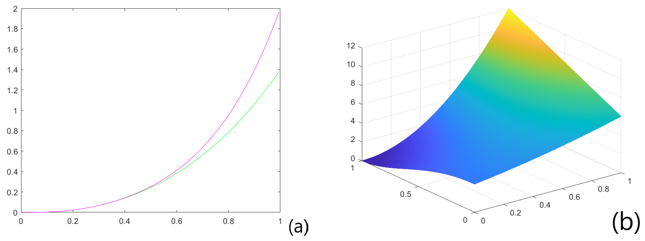
we find and The graphic of the function considered as function of two variables x and q, is given in Figure 1b. We see that the function is positive as .
One can see the validity of the inequality (3) in Figure 1a, where the green line in graph represents the expression of the left member of the inequality (3) and the expression of the right member represents the magenta line in graph.
We used here the Matlab R2023a software for obtaining Figure 1 and also partial in calculus of last two derivatives.
Example 2.
For the same function defined by , but with which satisfies the conditions of Theorem 4, we obtain for the left hand side of the inequality (3), by similar calculus, the expression,
Example 3.
Let consider the function defined by with which satisfies the conditions of Theorem 4. By calculus, under these hypothesis, we get for the left hand side of the inequality (3), the expression,
where we put and , obtaining,
By calculus we obtain,
On the other hand, by calculus, we have thus and Using that,
we find and The graphic of the function , considered as function of two variables x and q, is given in Figure 3b.
One can see the validity of the inequality (3) in Figure 3a, where the green line in graph represents the expression of the left member of the inequality (3) and the expression of the right member represents the magenta line in graph.
We used here the Matlab R2023a for obtaining Figure 3 and also partial in calculus of last two derivatives.
Example 4.
For the function defined by , but with which satisfies the conditions of Theorem 4, we obtain for the left hand side of the inequality (3), by similar calculus, the expression,
where we put and , obtaining,
On the other hand, by calculus, we have
thus by calculus, and from here, and We find, , and Therefore the right member becomes
and we have equality.
4. Discussion and Conclusions
The main findings of this study prove some new parametrized q-Hermite-Hadamard like type integral inequalities for functions whose second left and right q-derivative satisfies several different types of convexities. Some basic inequalities as q-Holder’s integral inequality and q-power mean inequality have been used in order to obtain the new estimated bounds. An auxiliary q-lemma was utilized as a main tool in our proofs. Symmetry can offer an advantage in study of many processes and phenomena from nature. Interesting consequences arise for special choices of the parameter and the corresponding cases were discussed in detail.
We used the Matlab R2023a software for figures and for some calculus in the examples. Several consequences, examples and applications were given to illustrate the outcome of the research.
Furthermore, it is interesting to extend such findings to other new kinds of convexities, -calculus, and q-fractional inequalities, which could be some good generalizations.
Even between the concept of convexity and the concept of symmetry there is a strong correlation, these two having many common ground to develop. This shows that the conclusions reached are pretty consistent. The study could be useful for the analysis of utility, distribution of taxes and revenues.
Overall, we hope that our results will improve the existing literature in the field.
Author Contributions
Conceptualization, L.C. and E.G.; methodology, L.C.; software, L.C.; validation, L.C. and E.G.; formal analysis, L.C.; investigation, L.C. and E.G.; resources, L.C. and E.G.; data curation, L.C.; writing—original draft preparation, L.C.; writing—review and editing, L.C. and E.G.; visualization, L.C. and E.G.; supervision, L.C. and E.G.; project administration, L.C. and E.G.; funding acquisition, L.C. and E.G. All authors have read and agreed to the version of the manuscript.
Funding
This research received no external funding.
Conflicts of Interest
The authors declare no conflict of interest.
References
- Awan, M.U.A.; Javed, M.Z.; Slimane, I.; Kashuri, A.; Cesarano, C.; Nonlaopon, K. (q1,q2)-trapezium like inequalities involving twice differentiable generalized m-convex functions and applications. Fractal Fract. 2022, 6, 435. [Google Scholar] [CrossRef]
- Xu, P.; Butt, S.I.; Ain, Q.U.; Budak, H. New Estimates for Hermite-Hadamard inequality in Quantum Calculus via (α,m) convexity. Symmetry 2022, 14, 1394. [Google Scholar] [CrossRef]
- Dragomir, S.S.; Khan, M.A.; Abathun, A. Refinement of the Jensen integral inequality. Open Math. 2016, 14, 221–228. [Google Scholar] [CrossRef] [Green Version]
- Dragomir, S.S. On Hadamard’s inequality for convex functions on the co-ordinates in a rectangle from the plane. Taiwan. J. Math. 2001, 5, 775–788. [Google Scholar] [CrossRef]
- Alomari, M.; Latif, M.A. On Hadamard-type inequalities for h-convex functions on the co-ordinates. Int. J. Math. Anal. 2009, 3, 1645–1656. [Google Scholar]
- Khan, A.; Chu, Y.M.; Khan, T.U.; Khan, J. Some inequalities of Hermite-Hadamard type for s-convex functions with applications. Open Math. 2017, 15, 1414–1430. [Google Scholar] [CrossRef]
- Alomari, M.; Darus, M.; Kirmaci, U.S. Some inequalities of Hermite-Hadamard type for s-convex functions. Acta Math. Sci. 2011, 31B, 1643–1652. [Google Scholar] [CrossRef]
- Kunt, M.; Iscan, I. Fractional Hermite-Hadamard-Fejer type inequalities for GA-convex functions. Turk. J. Inequal. 2018, 2, 1–20. [Google Scholar]
- Kalsoom, H.; Hussain, S. Some Hermite-Hadamard type integral inequalities whose n-times differentiable functions are s-logarithmically convex functions. Punjab Univ. J. Math. 2019, 51, 65–75. [Google Scholar]
- Al-Salam, W. Some fractional q-integrals and q-derivatives. Proc. Edinb. Math. Soc. 1966, 15, 135–140. [Google Scholar] [CrossRef]
- Toplu, T.; Kadakal, M.; Iscan, I. On n-polynomial convexity and some related inequalities. AIMS Math. 2020, 5, 1304–1318. [Google Scholar] [CrossRef]
- Ali, M.A.; Budak, H.; Murtaza, G.; Chu, Y.-M. Post-quantum Hermite-Hadamard type inequalities for interval-valued convex functions. J. Inequal. Appl. 2021, 2021, 84. [Google Scholar] [CrossRef]
- Jackson, F.H. On q-difference equations. Am. J. Math. 1910, 32, 305–314. [Google Scholar] [CrossRef]
- Agarwal, R. A propos d’une note de m. pierre humbert. Comptes Rendus l’Acad. Sci. 1953, 236, 2031–2032. [Google Scholar]
- Tariboon, J.; Ntouyas, S.K. Quantum calculus on finite intervals and aplications to impulsive difference equations. Adv. Differ. Equ. 2013, 2013, 282. [Google Scholar] [CrossRef] [Green Version]
- Tariboon, J.; Ntouyas, S.K. Quantum integral inequalities on finite intervals. J. Inequal. Appl. 2014, 13, 121. [Google Scholar] [CrossRef] [Green Version]
- Noor, M.; Noor, K.; Awan, M. Quantum Ostrowski inequalities for q-differentiable convex functions. J. Math. Inequal. 2016, 10, 1013–1018. [Google Scholar] [CrossRef]
- Alp, N.; Sarikaya, M.Z.; Kunt, M.; Iscan, I. q2-Hermite-Hadamard inequalities and quantum estimates for midpoint type inequalities via convex and quasi-convex functions. J. King Saud Univ. Sci. 2018, 30, 193–203. [Google Scholar] [CrossRef] [Green Version]
- Deng, Y.; Awan, M.U.; Wu, S. Quantum Integral Inequalities of Simpson-Type for Strongly Preinvex Functions. Mathematics 2019, 7, 751. [Google Scholar] [CrossRef] [Green Version]
- Bermudo, S.; Korus, P.; Valdes, J.N. On q-Hermite-Hadamard inequalities for general convex functions. Acta Math. Hung. 2020, 162, 364–374. [Google Scholar] [CrossRef]
- Khan, M.A.; Noor, M.; Nwaeze, E.R.; Chu, Y.M. Quantum Hermite-Hadamard inequality by means of a Green function. Adv. Difer. Equ. 2020, 2020, 99. [Google Scholar] [CrossRef]
- Kara, H.; Budak, H.; Alp, N.; Kalsoom, H.; Sarikaya, M.Z. On new generalized quantum integrals and related Hermite-Hadamard inequalities. J. Inequal. Appl. 2021, 2021, 180. [Google Scholar] [CrossRef]
- Latif, M.A.; Dragomir, S.S.; Momoniat, E. Some q-analogues of Hermite-Hadamard inequality of functions of two variables on finite rectangles in the plane. J. King Saud Univ. Sci. 2017, 29, 263–273. [Google Scholar] [CrossRef]
- Jhanthanam, S.; Tariboon, J.; Ntouyas, S.K.; Nonlaopon, K. On q-Hermite-Hadamard inequalities for differentiable convex functions. Mathematics 2019, 7, 632. [Google Scholar] [CrossRef] [Green Version]
- You, X.; Kara, H.; Budak, H.; Kalsoom, H. Quantum Inequalities of Hermite-Hadamard Type for r-Convex Functions. J. Math. 2021, 2021, 6634614. [Google Scholar] [CrossRef]
- Budak, H.; Ali, M.A.; Tarhanaci, M. Some New Quantum Hermite-Hadamard-Like Inequalities for Coordinated Convex Functions. J. Optim. Theory Appl. 2020, 186, 899–910. [Google Scholar] [CrossRef]
- Gulshan, G.; Hussain, R.; Budak, H. A new generalization of q-Hermite-Hadamard type integral inequalities for p,(p-s) and modified (p-s)-convex functions. Fract. Differ. Calc. 2022, 12, 147–158. [Google Scholar] [CrossRef]
- Chasreechai, S.; Ali, M.A.; Ashraf, M.A.; Sitthiwirattham, T.; Etemad, S.; De la Sen, M.; Rezapour, S. On New Estimates of q-Hermite-Hadamard Inequalities with Applications in Quantum Calculus. Axioms 2023, 12, 49. [Google Scholar] [CrossRef]
- Budak, H.; Erden, S.; Ali, M.A. Simpson and Newton inequalities for convex functions via newly defined quantum integrals. Math. Meth. Appl. Sci. 2020, 44, 378–390. [Google Scholar] [CrossRef]
- Ali, M.A.; Budak, H.; Zhang, Z.; Yildrim, H. Some new Simpson’s type inequalities for co-ordinated convex functions in quantum calculus. Math. Meth Appl. Sci. 2021, 44, 4515–4540. [Google Scholar] [CrossRef]
- Ali, M.A.; Abbas, M.; Budak, H.; Agarwal, P.; Murtazza, G.; Chu, Y.M. New quantum boundaries for quantum Simpson’s and quantum Newton’s type inequalities for preinvex functions. Adv. Differ. Equ. 2021, 2021, 64. [Google Scholar] [CrossRef]
- Vivas-Cortez, M.A.; Ali, M.A.; Kashuri, A.; Sial, I.B.; Zhang, Z. Some new Newton’s type integral inequalities for co-ordinated convex functions in quantum calculus. Symmetry 2020, 12, 1476. [Google Scholar] [CrossRef]
- Ali, M.A.; Chu, Y.M.; Budak, H.; Akkurt, A.; Yildrim, H. Quantum variant of Montgomery identity and Ostrowski-type inequalities for the mappings of two variables. Adv. Differ. Equ. 2021, 2021, 25. [Google Scholar] [CrossRef]
- Dragomir, S.S. Inequalities with applications in numerical analysis. AIP Conf. Proc. 2007, 936, 681. [Google Scholar]
- Srivastava, H.M.; Karlsson, P.W. Gaussian Hypergeometric Series; Halsted Press (Ellis Horwood Ltd.): Chichester, UK, 1985. [Google Scholar]
- Kalsoom, H.; Vivas-Cortez, M.; Abidin, M.Z.; Marwan, M.; Khan, Z.A. Montgomery identity and Ostrowski-type inequalities for generalized quantum calculus through convexity and their applications. Symmetry 2022, 14, 1449. [Google Scholar] [CrossRef]
- Alp, N.; Budak, H.; Sarikaya, M.Z.; Ali, M.A. On new refinements and generalizations of q-Hermite-Hadamard inequalities for convex functions. Rocky Mt. J. Math. 2023. Available online: https://projecteuclid.org/journals/rmjm/rocky-mountain-journal-of-mathematics/DownloadAcceptedPapers/220708-Budak.pdf (accessed on 4 June 2023).
- Ciurdariu, L.; Grecu, E. Several quantum Hermite-Hadamard type integral inequalities for convex functions. Fractal Fract. 2023, 7, 463. [Google Scholar] [CrossRef]
- Luangboon, W.; Nonlaopon, K.; Tariboon, J.; Ntouyas, S.K.; Budak, H. Post-Quantum Ostrowski type integral inequalities for twice (p,q)-differentiable functions. J. Math. Ineq. 2022, 16, 1129–1144. [Google Scholar] [CrossRef]
- Ciurdariu, L.; Grecu, E. Post-quantum integral inequalities for three-times (p,q)-differential functions. Symmetry 2023, 246, 15. [Google Scholar]
- Bleichrodt, H.; Van Doorslaer, E. A welfare economics foundation for health inequality measurement. J. Health Econ. 2006, 25, 945–957. [Google Scholar] [CrossRef] [Green Version]
- Fare, R.; Grosskopf, S. Notes on some inequalities in economics. Econ. Theory 2000, 15, 227–233. [Google Scholar] [CrossRef]
- Mathews, T.; Schwartz, J.A. Comparisons of utility inequality and income inequality. Econ. Lett. 2019, 178, 18–20. [Google Scholar] [CrossRef]
- Khan, M.A.; Anwar, S.; Khalid, S.; Sayed, Z.M.M.M. Inequalities of the type Hermite-Hadamard-Jensen-Mercer for strong convexity. Math. Probl. Eng. 2021, 2021, 5386488. [Google Scholar]
- Chu, Y.-M.; Awan, M.U.; Talib, S.; Noor, M.A.; Noor, K.I. New post quantum analogues of Ostrowski-type inequalities using new definitions of left-right (p,q)-derivatives and definite integrals. Adv. Differ. Equ. 2020, 2020, 634. [Google Scholar] [CrossRef]
- Kalsoom, H.; Vivas-Cortez, M.; Latif, M.A. Trapezoidal-Type inequalities for strongly convex and quasi-convex via post-quantum calculus. Entropy 2021, 23, 1238. [Google Scholar] [CrossRef] [PubMed]
- Ion, D.A. Some estimates on the Hermite-Hadamard inequality through quasi-convex functions. Ann. Univ. Craiova Ser. Mat. Inform. 2007, 34, 83–88. [Google Scholar]
- Hadamard, J. Etude sur les proprietes des fonctions entieres en particulier d’une fonction consideree par Riemann. J. Math. Pures. Appl. 1893, 58, 171–215. [Google Scholar]
- Gasper, G.; Rahman, M. Basic Hypergeometric Series, 2nd ed.; Encyclopedia of Mathematics and Its Applications; Cambridge University Press: Cambridge, UK, 2004; Volume 96. [Google Scholar]
- Rajkovic, P.M.; Stankovic, M.S.; Marinkovic, S.D. The zeros of polynomials orthogonal with respect to q-integral on several intervals in the complex plane. In Proceedings of the Fifth International Conference of Geometry Integrability and Quantization, Varna, Bulgaria, 5–12 June 2003; pp. 178–188. [Google Scholar]
- Ernst, T.A. Comprehensive Treatment of q-Calculus; Springer: Basel, Switzerland, 2012. [Google Scholar]
- Kac, V.; Cheung, P. Quantum Calculus; Springer: New York, NY, USA, 2003; 652p. [Google Scholar]
Figure 1.
(a) An example for the inequality (3) from Theorem 4 for the function and , when ; (b) Graphic for the functions , considered as function of two variables x and q, from Example 1 when , , and .
Figure 1.
(a) An example for the inequality (3) from Theorem 4 for the function and , when ; (b) Graphic for the functions , considered as function of two variables x and q, from Example 1 when , , and .

Figure 2.
An example for the inequality (3) from Theorem 4 for the function and , when .
Figure 2.
An example for the inequality (3) from Theorem 4 for the function and , when .

Figure 3.
(a) An example for the inequality (3) from Theorem 4 for the function , and ; (b) Graphic for the function from Example 3, considered as function of two variable x and q, when , , and .
Figure 3.
(a) An example for the inequality (3) from Theorem 4 for the function , and ; (b) Graphic for the function from Example 3, considered as function of two variable x and q, when , , and .

Disclaimer/Publisher’s Note: The statements, opinions and data contained in all publications are solely those of the individual author(s) and contributor(s) and not of MDPI and/or the editor(s). MDPI and/or the editor(s) disclaim responsibility for any injury to people or property resulting from any ideas, methods, instructions or products referred to in the content. |
© 2023 by the authors. Licensee MDPI, Basel, Switzerland. This article is an open access article distributed under the terms and conditions of the Creative Commons Attribution (CC BY) license (https://creativecommons.org/licenses/by/4.0/).
Share and Cite
MDPI and ACS Style
Ciurdariu, L.; Grecu, E. New Perspectives of Symmetry Conferred by q-Hermite-Hadamard Type Integral Inequalities. Symmetry 2023, 15, 1514. https://doi.org/10.3390/sym15081514
AMA Style
Ciurdariu L, Grecu E. New Perspectives of Symmetry Conferred by q-Hermite-Hadamard Type Integral Inequalities. Symmetry. 2023; 15(8):1514. https://doi.org/10.3390/sym15081514
Chicago/Turabian StyleCiurdariu, Loredana, and Eugenia Grecu. 2023. "New Perspectives of Symmetry Conferred by q-Hermite-Hadamard Type Integral Inequalities" Symmetry 15, no. 8: 1514. https://doi.org/10.3390/sym15081514
Note that from the first issue of 2016, this journal uses article numbers instead of page numbers. See further details here.