
An Alternate Generalized Odd Generalized Exponential Family with Applications to Premium Data
by
 , , , and
Sadaf Khan
1,* ,
,
Oluwafemi Samson Balogun
2,*,
Muhammad Hussain Tahir
1,
Waleed Almutiry
3 and
Amani Abdullah Alahmadi
4 1
Department of Statistics, The Islamia University of Bahawalpur, Bahawalpur 63100, Pakistan
2
School of Computing, University of Eastern Finland, 70211 Kuopio, Northern Europe, Finland
3
Department of Mathematics, College of Science and Arts in Ar Rass, Qassim University, Buryadah 52571, Saudi Arabia
4
College of Science and Humanities, Shaqra University, Shaqra 15572, Saudi Arabia
*
Authors to whom correspondence should be addressed.
Symmetry 2021, 13(11), 2064; https://doi.org/10.3390/sym13112064
Submission received: 19 September 2021
/
Revised: 14 October 2021
/
Accepted: 14 October 2021
/
Published: 1 November 2021
(This article belongs to the Special Issue Symmetric Distributions, Moments and Applications)
Abstract
:In this article, we use Lehmann alternative-II to extend the odd generalized exponential family. The uniqueness of this family lies in the fact that this transformation has resulted in a multitude of inverted distribution families with important applications in actuarial field. We can characterize the density of the new family as a linear combination of generalised exponential distributions, which is useful for studying some of the family’s properties. Among the structural characteristics of this family that are being identified are explicit expressions for numerous types of moments, the quantile function, stress-strength reliability, generating function, Rényi entropy, stochastic ordering, and order statistics. The maximum likelihood methodology is often used to compute the new family’s parameters. To confirm that our results are converging with reduced mean square error and biases, we perform a simulation analysis of one of the special model, namely OGE2-Fréchet. Furthermore, its application using two actuarial data sets is achieved, favoring its superiority over other competitive models, especially in risk theory.
1. Introduction
In recent years, there has been a dramatic growth in the number of generalisations of well-known probability distributions. Most notable generalizations are achieved by (i) inducting power parameters in well established parent distributions, (ii) extending the classical distribution by modification in their functions, (iii) introducing special functions such as W[K(x)] as generators and (iv) by compounding of distributions. This heaped surge of generalized families is due to the flexibility in modelling phenomenons related to the changing scenarios of contemporary scientific field including demography, actuarial, survival, biological, ecological, communication theory, epidemiology and environmental sciences. However, a clear understanding of the applicability of these models in most applied areas is necessary if one is to gain insights into systems that can be modeled as random processes. The model, thus obtained, acquires improved empirical results to the real data that is collected adaptively.
Although there exist many functions which act as generators to produce flexible classes of distributions, in this project, we will emphasize generalizations in which a ratio of survival function (sf) has been used in some form, commonly known as the odd ratio. In the reference [1], a proportional odd family viz. a viz. the Marshall Olkin-G (MO-G) was generalized by sf , where is the distribution function (cdf) of parent distribution, with the induction of a tilt parameter. Gleaton and Lynch, in the reference [2], used the odd function as generator when they defined a log odd family (OLL-G). In the reference [3], defined the odd Weibull family, as an asymptotically equivalent log-logistic model for larger values of , the scale parameter. The reference [4] used the Transformed -Transformer (TX) family, due to the reference [5], to define odd Weibul-G families of distribution. Since then, a myriad of distributions has been generalized using odd function. Some of the important families include [6,7,8,9,10,11,12,13,14,15,16,17,18,19,20,21,22,23,24,25,26,27,28,29,30,31], among others.
Focussing on the origins and motivations of our proposed scheme, the authors in [32] proposed the odd generalized exponential family (which we refer to OGE-G) as a better alternative to generalized exponential (GE) family using Lehmann Alternative-I (LA-I). The cdf of the two parameter OGE-G family is mentioned below:
In the reference [33], an odd family of GE was proposed so-called generalized odd generalized exponential family (which we refer to OGE1-G). The cdf of OGE1-G family is presented as:
Because of its capacity to simulate variable hazard rate function (hrf) forms of all traditional types in lifetime data analysis, we believe OGE-G offers a sensible combination of simplicity and flexibility. However, the relevance of OGE1-G to lifespan modelling in domains such as reliability, actuarial sciences, informatics, telecommunications, and computational social sciences (just to highlight a few) is still debatable. According to the reference [34], the Lehmann Alternative-II (LA2) approach has received less attention. This motivated us to use LA2 approach to develop the exponentiated odd generalized exponential (OGE2-G), in the same vein as OGE-G and OGE1-G. Adhering to the framework defined in the reference [5], if T follows GE random variable (rv), then the cdf of OGE2-G family is mentioned below:
where and are shape parameter and is the vector of baseline parameter.
Consider the following points to emphasise the model’s distinctiveness; (i) In the literature, the proposed model in its current form has not been studied to the best of our knowledge, (ii) From an analytical standpoint, the OGE2-G family has a significantly better configuration and practicality than OGE-G and OGE1-G for inverted models with minimal chance to counter non-identifiability issues, (iii) The OGE2-G has several curious connections to other families. When approaches 0, tends to GE with , when tends to OGE-G, if and then tends to odd exponential (OE) (iv) This new dimension allowed us to explore models which are naturally constituted by LA2. The generalizations, thus attained, produced skewed distributions with much heavier tails enabling its practicality in risk evaluation theory with far better results, (v) The successful application of OGE2-G family motivates future research, as it outperforms nine well-established existing models, (vi) We present a physical explanation for X when and are integers. Consider there be a parallel system consisting of identically independent components. Suppose that the lifetime of a rv Y with a specific with components in a series system such that the risk of failing at time x is represented by the odd function as . Consider that the randomness of this risk is represented by the rv X, then we can assume the following relation holds
explicitly given in Equation (1). The OGE2-G family is offered and explored in this research, emphasising its diversity and scope for application to real life phenomenons. The major features of the OGE2-G family, including the pdf, hrf, qf, and ten unique models from OGE2-G family presented in Table 1, are provided in the first half. Then, certain mathematical properties of the OGE2-G such as series expansion of the exponentiated pdf, moments, parameter estimation, order statistics, Rényi entropy, stress-strength analysis and stochastic dominance results are investigated. Furthermore, Fréchet is specified as baseline model termed as OGE2-Fréchet (denoted as OGE2Fr) and the maximum likelihood (ML) technique is then used to construct statistical applications of the special model. We choose to study OGE2Fr specifically as its nested model include inverse-Rayleigh (IR) and inverse exponential (IE), favoring its suitability over sub-models as well. It is applied to fit two sets of premium data from actuarial field. Using key performance indicators, we reveal that OGE2Fr outperforms nine competing models. A portion pertinent to specific risk measures, with an emphasis on the value at risk (VaR) and the expected shortfall (ES), is presented. Eventually, the estimation of risk measures for the examined data sets is then discussed, with the proposed methodology yielding a rather satisfying result. Equation (1) can be useful in modelling real life survival data with different shapes of hrf. Table 1 lists and the corresponding parameters for some special distributions which are considered to be the potential sub-models of OGE2-G family.
The following is a breakdown of how the paper is constructed. In Section 2, we acquaint the readers to the new family with basic properties and ten potential baseline models which can become members of OGE2-G family. Section 3 is comprised of the mathematical properties of the OGE2-G family. Section 4 progresses by taking Fréchet (Fr) as sub-model to propose OGE2Fr and related statistical and inferential properties. Section 5 specifies two applications of actuarial data sets with emphasis on risk evaluation (premium returns) and the proposed model’s veracity is established. Furthermore, the model is applied to compute some actuarial measures. Section 6 is the final section, with some annotations and useful insights.
2. The OGE2G Family
In this segment, basic statistical properties of the newly proposed family characterized by the cdf, in Equation (1) are presented. Functional forms of ten sub models are also defined.
2.1. Definition of pdf and hrf
The hazard rate is just a calculation of the change in survivor rate per unit of time. Hence, its importance in reliability and survival analysis is crucial. The hrf has some characteristic shapes which include monotonic (increasing, decreasing), non-monotonic (bathtub or upside down bathtub) or constant. Standard statistical distribution yield maximum three shapes, but OGE2-G family can yield a diverse range of shapes (including increasing-decreasing-increasing) depending upon the choice of special model. For further details on hrf, see [35].
2.2. Quantile Function and Potential Sub-Models
The OGE2-G family may be readily approximated by reversing Equation (1) as shown below: If indeed the distribution of u is uniform , therefore
Equation (4) can be useful to define statistical measures such as median, skewness, and kurtosis based on quartiles, deciles, or percentiles. These measures facilitates to concisely define the skewness and kurtosis measures which are significant tool to comprehend the shape(s) of the distribution.
Theorem 1 shows how the OGE2 family is related to other distributions.
Theorem 1.
Let , then
(a) If Y = , then , and
(b) If Y = , then .
3. Mathematical Properties of OGE2-G Family
To capture the family’s modelling capacity, numerous mathematical features of the OGE2-G are examined in this section. Some of the key results established in this section are then applied in Section 5.
3.1. Linear Expansion of cdf
We provide a useful expansion for (1) in terms of linear combinations of exp-G density functions using the following series expansion as
whereas the expansion holds for all and a non-integer value. Then, the cdf of OGE2-G class in (1) can indeed be phrased with
Using series expansion and power series expansion in Equation (5), will yield the following cdf
where (for ) denotes the cdf of exp-G distribution with power parameter ℓ and
Through differentiating Equation (6) the OGE2-G family density, we may express it as a combination of exp-G densities.
where is the exp-G pdf with power parameter ℓ. As a result, numerous features of the proposed model may be deduced from the exp-G distribution’s attributes. Most modern computation frameworks, such as MathCad, Maple, Mathematica, and Matlab, can efficiently handle the formulas derived throughout the article, which can currently operate using the use of analytic formulations of enormous size and complexity.
3.2. Numerous Types of Moments
The fundamental formula for the pth moment of X is supplied by (7) as
where Setting in (8) can provide explicit expression for the mean of several parent distributions.
A another expression for is taken from (8) as far as the baseline qf is concerned
where
The central moments () and cumulants () of X can follow from Equation (8) as and , respectively, where .
For most G distributions, the final integral may be calculated.
3.3. Inference Related to OGE2 Family
The strategy of maximum likelihood (MLL) approach is used to estimate the unknown parameters of the new class. Let be n observations from the OGE2-G density class (2) with parameter vector . Then the likelihood function on the domain is defined as
where = .
The elements of the score vector are as described in the following:
where and means the derivative of the function V with respect to and , respectively.
The next elements are produced by the components of the score vector .
where is the derivative of with respect to , is the derivative of with respect to and is the derivative of with respect to .
3.4. Entropy
The Rényi entropy due to [36], is characterized as
Let us consider
3.5. Order Statistics
Assume that is a random sample (RS) from the OGE2-G. Furthermore, assume that denote the ith order statistic (OS). Consequently, pdf of may be interpreted as
Inserting Equations (1) and (2) in the last equation, and expanding it as in Section 3.1, we get
where
and
3.6. Stress-Strength Reliability
Supp and are two continuous rvs with pdfs and and cdfs and , therefore the reliability R is supplied via
Theorem 2.
Assume that and are two independent rvs established previously with constant parameters and . Eventually,
3.7. Stochastic Ordering
Stochastic ordering has indeed been acknowledged as an essential tool for assessing comparative behavior in reliability theory and other disciplines. Assume X and Y be two rvs via cdfs, sfs and pdfs and , and , and and , respectively. In the specific planning, the rv is considered to be lower than :
- Stochastic order (symbolized via ) if for all x;
- LL ratio order (symbolized via ) if is decreasing in ;
- Hazard rate order (symbolized via ) if is decreasing in ;
- Reversed hazard rate order (symbolized via ) if is decreasing in .
All these four stochastic orders studied in (1)–(4) are connected to one another as a result of [37] and the accompanying ramifications apply:
when sufficient conditions are met, the OGE2-G distributions are ordered with regard to the strongest LL ratio ordering, as shown by the next theorem.
Theorem 3.
Assume and . If , then
Proof.
First, we have the ratio
After simplification, we obtain
Next,
If , we obtain
Thus, is decreasing in x and hence . □
4. OGE2-Fréchet Distribution
In this section, we study the first special model defined in Section 2.2, the OGE2-Fréchet (OGE2Fr), in view of its practical application.
The OGE2Fr model can be defined from (1) by taking and , as cdf and pdf of the baseline Fréchet distribution with , respectively. The cdf and pdf of OGE2Fr distribution are, respectively, given by
and
where and b are shape parameters while a is scale parameter.
The hrf and qf of the OGE2Fr distribution are obtained as
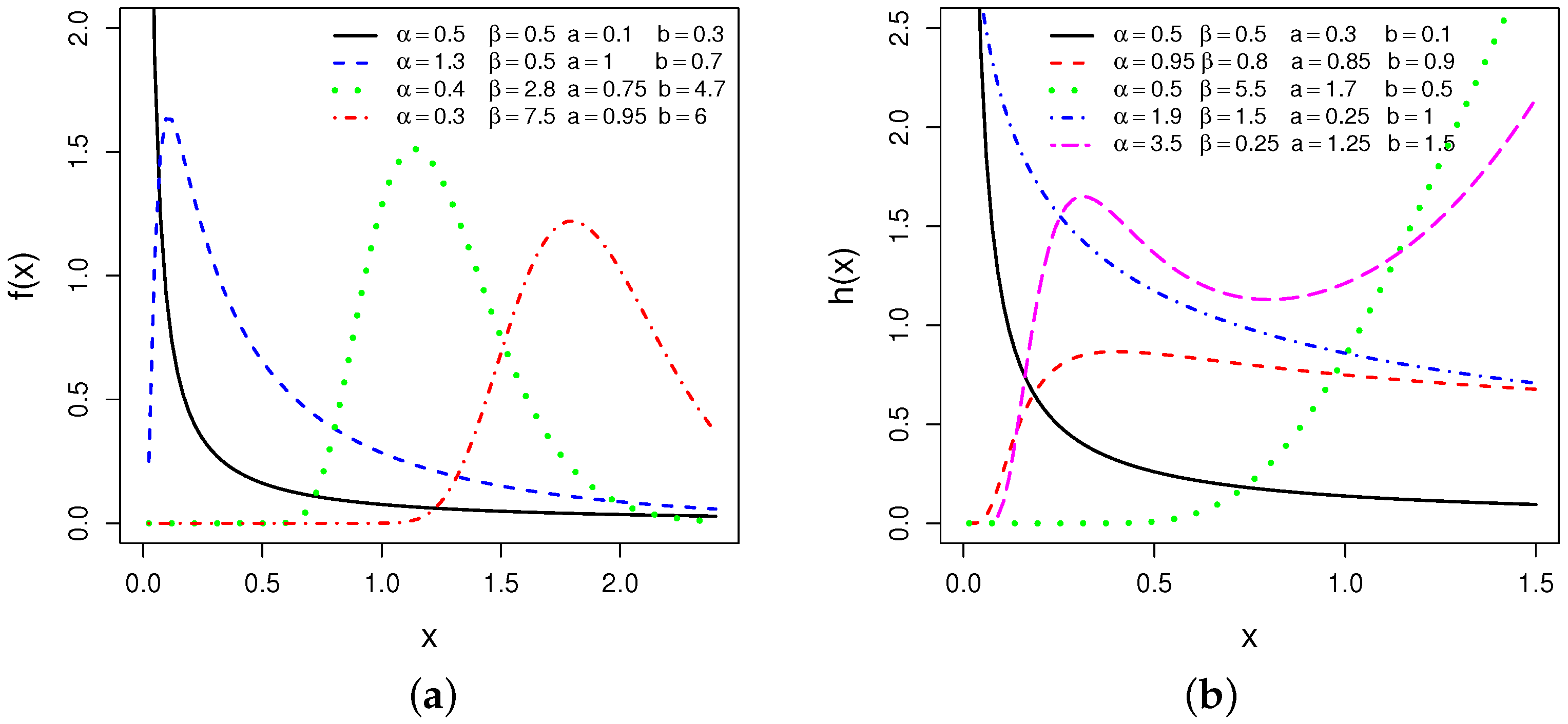
Figure 1 depicts a visualisation of the pdf and hrf functions, exhibiting the range of shapes that all these functions can take at random input parametric values. The OGE2Fr distribution’s pdf can be gradually decreasing, unimodal, and right-skewed, with different curves, tail, and asymmetric aspects, as shown in Figure 1. The hrf, on the other hand, offers an extensive range of increasing, decreasing, unimodal, and increasing-decreasing-increasing (IDI) forms. Given a wide variety of hrf shapes being offered, the OGE2Fr distribution can in fact be a useful tool to model unpredictable time-to-event phenomena.
4.1. Linear Representation and Related Properties
The cdf of the OGE2Fr distribution is quite straightforward and is achieved by using the result defined in Equation (6) as
where ℓ is the power parameter and noting that is unity.
For simplicity, we can rewrite the above result as
By differentiating the last term, we can express the density of OGE2Fr model as follows
where represents the Fréchet density function with power parameter ℓ. Equation (22) enforces the fact that OGE2Fr density is a linear combination of Fréchet densities. Thus, we can derive various mathematical properties using Fréchet distribution.
Moments are the heart and soul of any statistical analysis. Moments can be used to evaluate the most essential characteristics such as mean, variance, skewness, and kurtosis of a distribution. We now directly present the mathematical expressions for the moments of OGE2Fr model as follows. Let be a random variable with density . Then, core properties of X can follow from those of . First, the pth ordinary moment of X can be written as
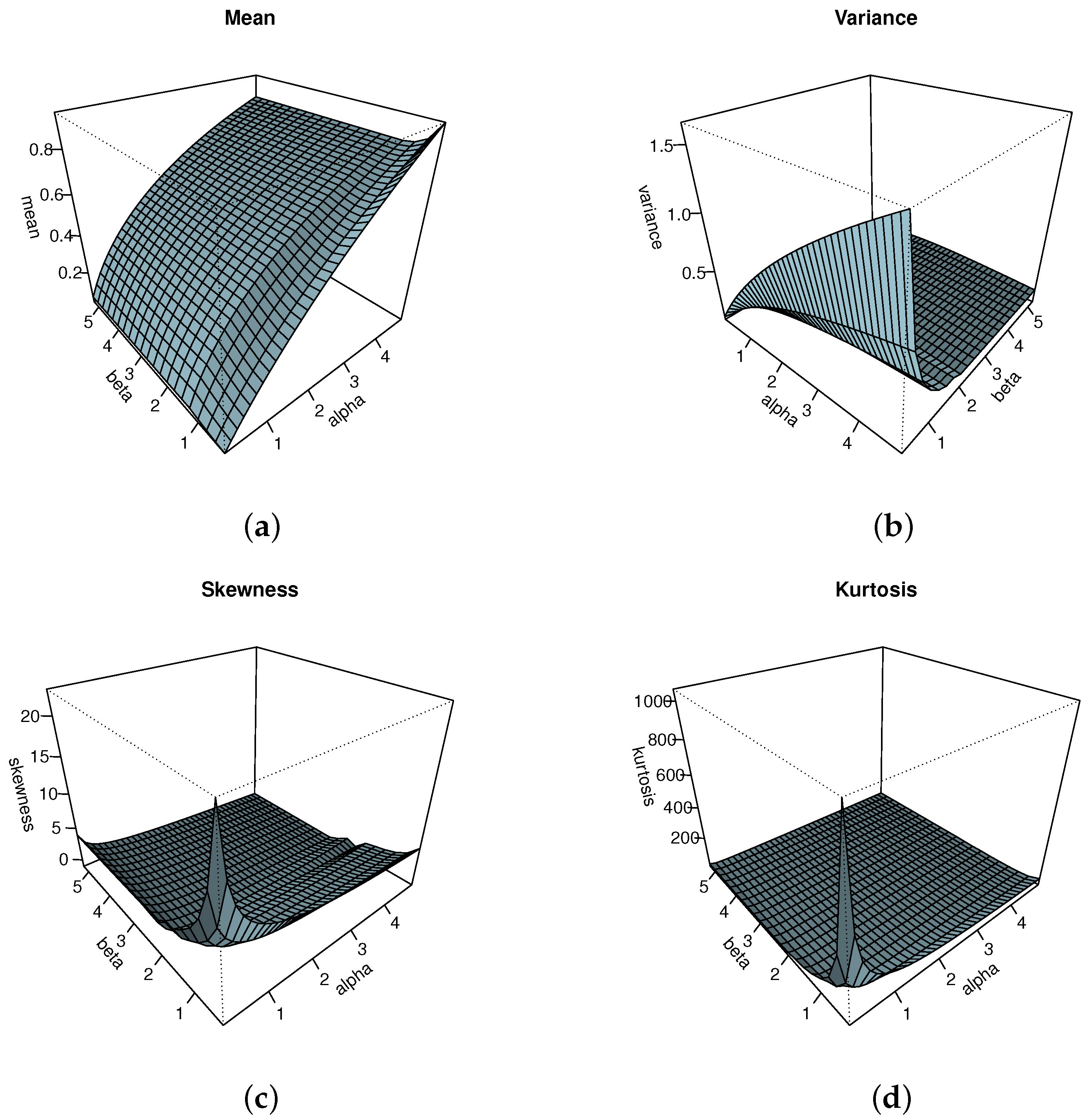
Second, the cumulants () of X can be determined recursively from (23) as , respectively, where . The skewness and kurtosis of X can be calculated from the third and fourth standardized cumulants. Plots of mean, variance, skewness and kurtosis of the OGE2Fr distribution are displayed in Figure 2. These plots signifies the significant role of the parameters and in modeling the behaviors of X.
Third, the pth incomplete moment of X, denoted by , is easily found changing variables from the lower incomplete gamma function when calculating the corresponding moment of . Then, we obtain
Fourth, the first incomplete moment is used to construct the Bonferroni and Lorenz curves as discussed in Section 3.2. Figure 3 provides the income inequality curves (Bonferroni & Lorenz) of the proposed distribution which can easily be derived from (24), respectively, where is the qf of X derived from Equation (20).
4.2. Parameter Estimation
Let be a sample of size n from the OGE2Fr distribution given in Equation (18). The log-likelihood function for the vector of parameters is -4.6cm0cm
The components of score vectors U() are
4.3. Order Statistics
For a random sample of taken from the OGE2Fr distribution with as the ith order statistic. For , the pdf corresponding to can be expressed as
where and are the pdf and cdf of OGE2Fr distribution, respectively. Inserting Equations (17) and (18), and using the result defined in Section 3, we have
where
and
is the probability density function of the OGE2Fr distribution with parameters and b.
4.4. Stochastic Ordering
In several areas of probability and statistics, stochastic ordering and disparities are being adhered to at an accelerating rate. For example, in analyzing the contrast of investment returns to random cash flows; two manufacturers may use distinct technologies to make gadgets with the same function, resulting in non-identical life distributions or comparing the strength of dependent structures. Here, we use the term stochastic ordering to refer to any ordering relation on a space of probability measures in a wide sense. Let X and Y be two rvs from OGE2Fr distributions, with assumptions previously mentioned in Section 3. Given that , and for , shall be decreasing in x if and only if the following result holds Let X and Y be two rvs from OGE2Fr distributions, with assumptions previously mentioned in Section 3. Given that , and for , shall be decreasing in x if the following result holds
4.5. Simulation Study
By using the result defined in Equation (25), we evaluate the sensitivity of the method of estimations using the MLEs of OGE2Fr distribution parameters by Monte Carlo simulation technique. The simulation study is conducted for sample sizes and parameter combinations, denoted by , are:
- : , , and ;
- : , , and ;
- : , , and .
We use Equation (20) to generate the random observations. For each , the empirical bias and MSE values are the average of the values from simulated samples for given sample size n. The formula to evaluate the mean squared error (MSEs) and the average bias (Bias) of each parameter, is given below
We report the results of the AE, Bias and MSE for the parameters , , a and b in Table 2. The MSE of the estimators increases when the assumed model deviates from the genuine model, as anticipated. When the sample size grows larger and the symmetry degrades, the MSE shrinks. Generally speaking, the MSE decreases when the kurtosis grows. Similarly, when the asymmetry rises, the bias grows, and vice versa. As the kurtosis grows, the bias becomes smaller. In conclusion, it is apparent that the MSEs and Biases decrease when the sample size n increases. Thus, we can say that the MLEs perform satisfactorily well in estimating the parameters of the OGE2Fr distribution.
5. Application of OGE2Fr to Premium Data
Most skewed distributions are suitable to measure risk measures associated with actuarial data. The risks involve credit, portfolio, capital, premiums losses, and stocks prices among others. We focus our attention on the stakes based on premiums. Premiums are the payments for insurance that the customer pay to the company to which they are insured. In this section, we apply the OGE2Fr lifetime model for the statistical analysis of two real life data sets both of which include premium losses. Our aim is to compare the fits of the OGE2Fr model with other well-known generalizations of the Fréchet (Fr) models given in Table 3.
The first premium data set, designated as PD1, is derived from complaints upheld against vehicle insurance firms as a proportion of their overall business over a two-year period. The study was conducted by DFR (Darla Fry Ross) insurance and investment company (2009–2016), registered in New York state. The most common complaints are over delays in the settlement of no-fault claims and non-renewal of insurance. Top of the list are insurers with the fewest upheld complaints per million USD of premiums. The companies with the greatest complaint ratios are at the bottom of the list. The data understudy is from the year 2016. The second premium data, denoted by PD2, signifies the net premiums written (in billions of USD) to insurers which, under Article 41 of the New York Insurance Law, are required to meet minimum financial security requirements. Table 4: Descriptives statistics of PD1 and PD2.
The OGE2Fr model is validated through the discriminatory criterions (DCs) we considered for each data set. It includes the negative log-likelihood () of the model taken at the corresponding MLEs, the Akaike Information Criterion (AICs), Bayesian Information Criterion (BICs), Anderson-Darling (AD), Cramér–von Mises (CvM), and Kolmogrov-Smirnov (KS) as well as the p-value (P-KS) of the related KS test. We use the method of maximum likelihood estimation to estimate the unknown parameters as presented in Section 4.2. For each criterion (except p-value (KS)) with highest value), the smallest values is gained by the OGE2Fr model, indicating the best fit among its competitive models.
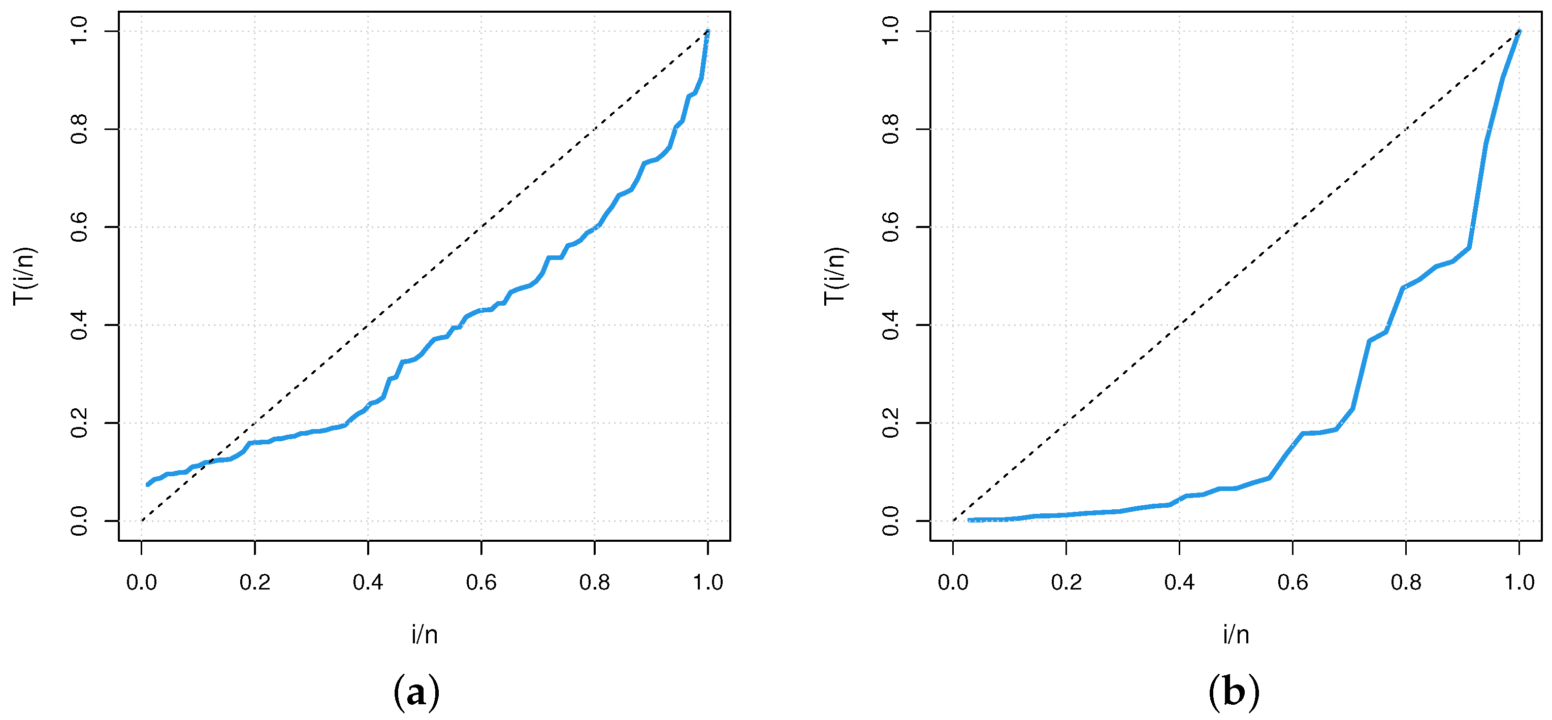
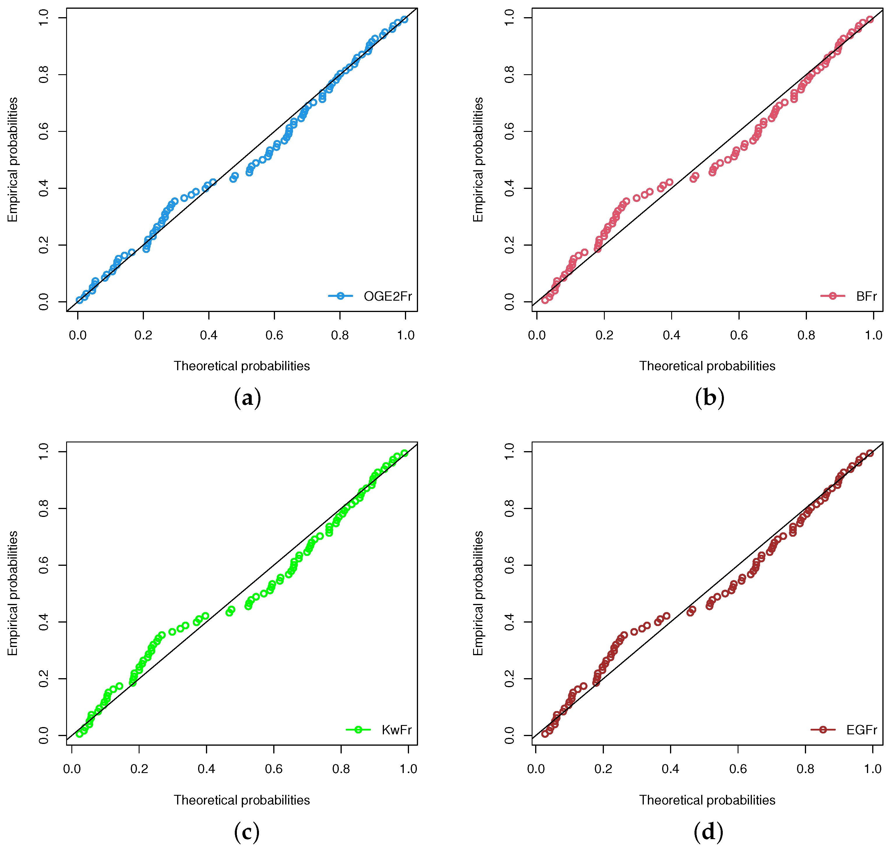
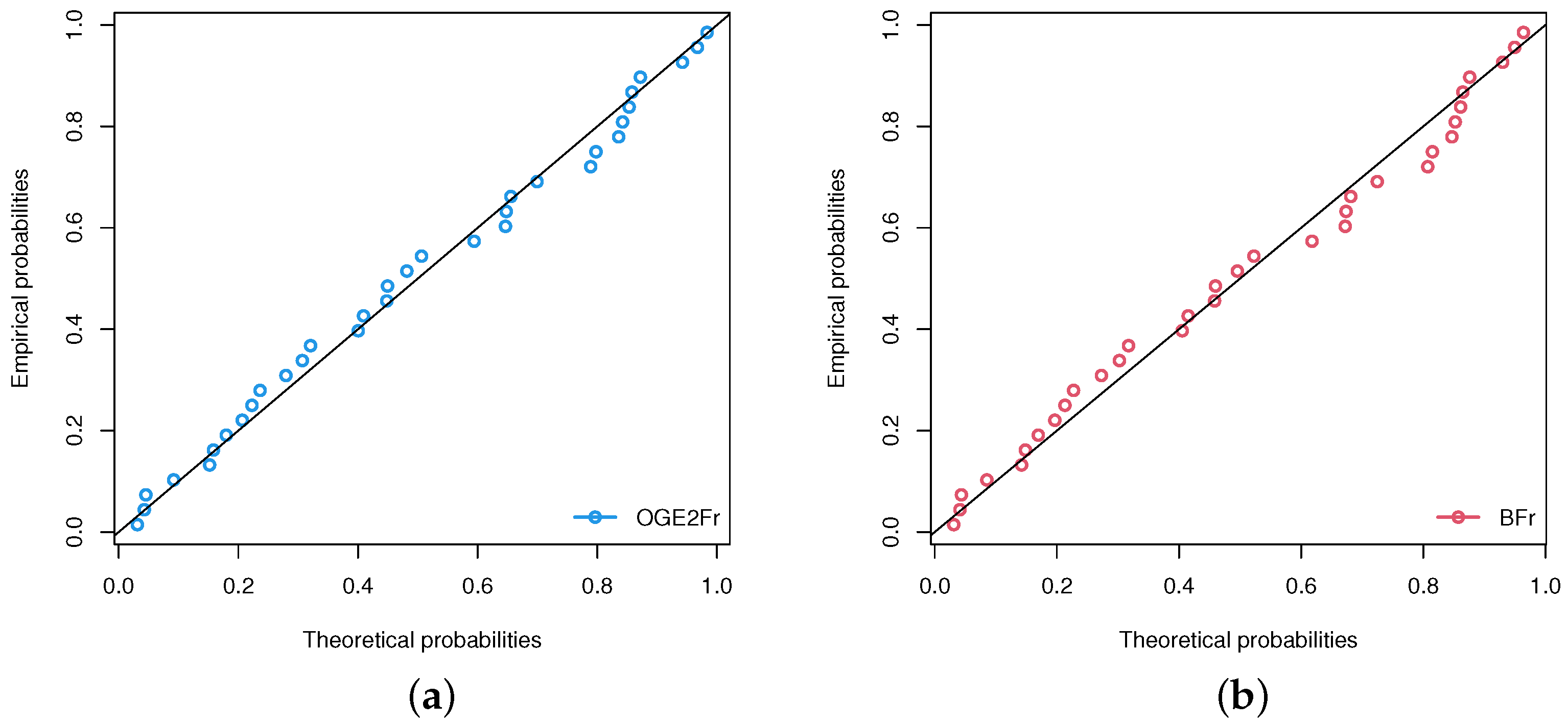
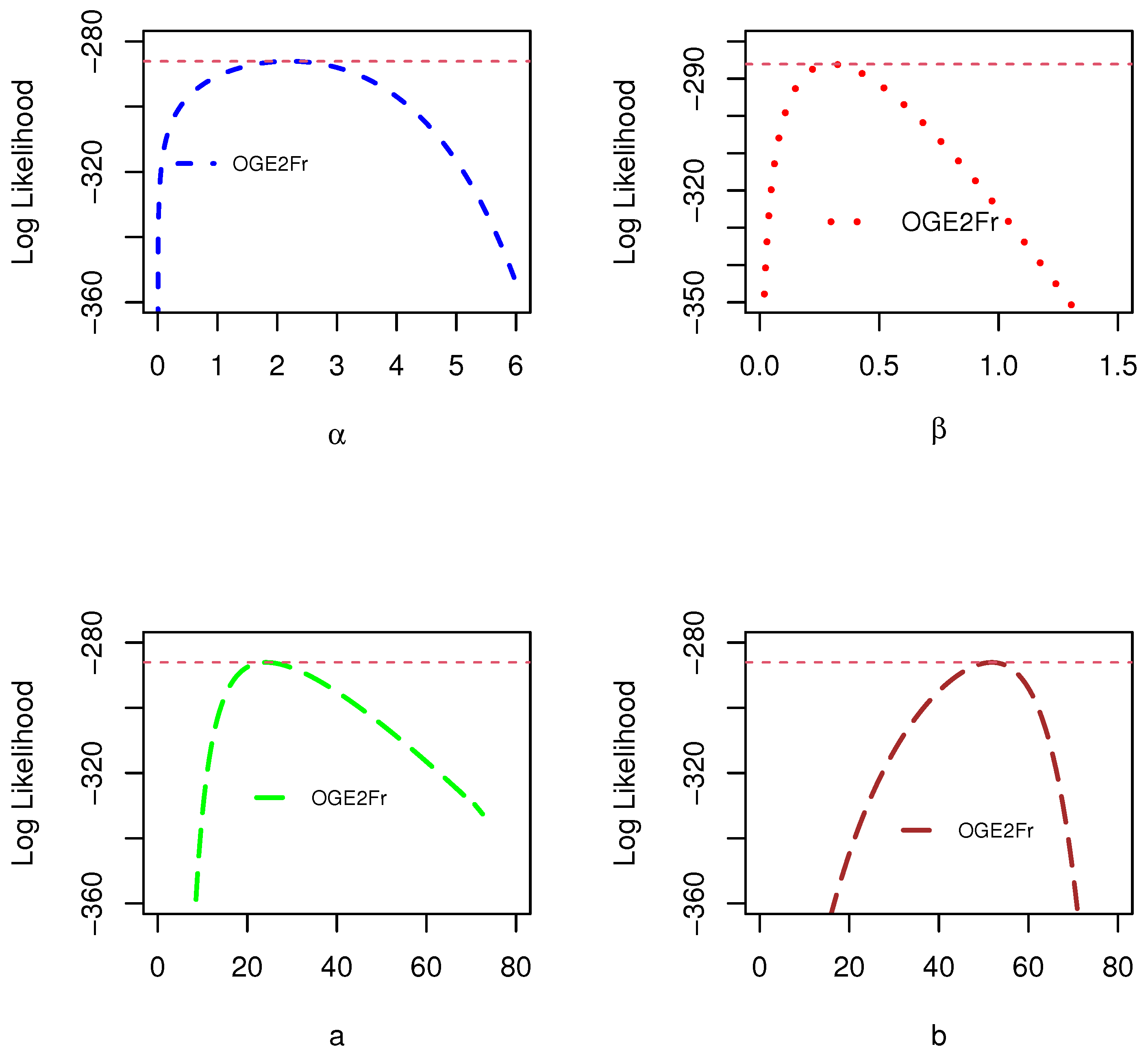
Some descriptive statistics related to these data are given in Table 4. The skewness and kurtosis are indicative of exponentially tailed data (reversed-J shape). The TTT plots for the both data sets are given in Figure 4. In particular, the TTT plots show largely decreasing hrf, permitting to fit OGE2Fr model on these data sets. The estimated hrf in Figure 5 matches Figure 4. In Table 5, we present the estimates (MLEs) along with their respective standard errors(SEs) while the DCs are listed in Table 6 for PD1 & PD2, respectively. For a more visual view, the estimated pdf, cdf, sf and Q-Q plots of the OGE2Fr model for two data sets are displayed in Figure 6 and Figure 7. Furthermore, the PP-plots of OGE2Fr and its three other competitive 4-parameter models for PD1 and PD2 are displayed in Figure 8 and Figure 9. The log-likelihood function profiles for PD1 and PD2, respectively, are provided in Figure 10 and Figure 11 to highlight the universality of the MLEs of vector. The graphical visualizations are indicative of nice fits for the OGE2Fr model.
5.1. Actuarial Measures
One of the most important duties of actuarial sciences organizations is to assess market risk in a portfolio of instruments, which originates from changes in underlying factors such as equities prices, interest rates, or currency rates.One of the most important duties of actuarial sciences organizations is to assess market risk in a portfolio of instruments, which originates from changes in underlying factors such as equities prices, interest rates, or currency rates. We compute several important risk measures for the suggested distribution in this section, such as Value at Risk (VaR) and Expected Shortfall (ES), which are important in portfolio optimization under uncertainty.
5.1.1. Value at Risk
The quantile premium principal of the distribution of aggregate losses, commonly known as Value at risk (VaR), is the most widely used measure to evaluate exposure to risk in finance. VaR of a rv is the pth quantile of its cdf. If OGE2Fr denotes a random variable with cdf (17), then its VaR is
5.1.2. Expected Shortfall
Artzner et al. [47,48] recommended the use of conditional VaR instead of VaR, famously called Expected Shortfall (ES). The ES is a metric that quantifies the average loss in situations where the VaR level is exceeded. It is defined by the following expression
The ES of OGE2Fr is given by
Figure 12 illustrates VaR and ES for some random parameter combinations of OGE2Fr.
5.1.3. Numerical Calculation of VaR and ES
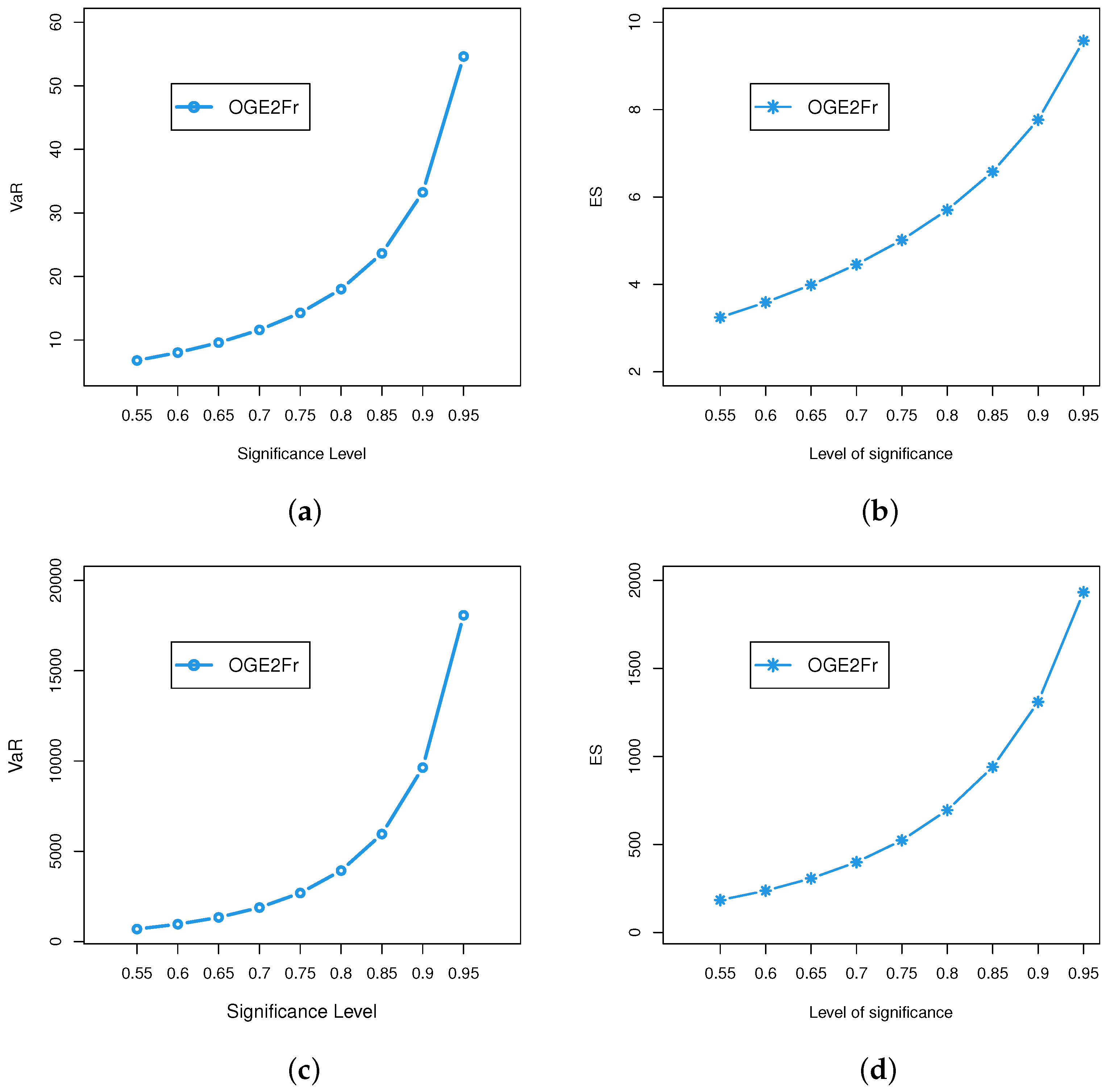
The results of OGE2Fr presented in Section 4 allowed us to further explore its application to these risk measures. From Table 5, we take the values of MLEs of PD1 and PD2, respectively, to measure the volatility associated with these measures. Higher values of these risk measures signify heavier tails while lower values indicate a much lighter tail behavior of the model. It is worth mentioning that the OGE2Fr model produced substantially more significant results than its counterparts, indicating that the model has a heavier tail. In Table 7, we show the numerical results of VaRs and ESs of PD1 and PD2, respectively, of the proposed model. For the convenience of the reader, Figure 13 show the results graphically.
6. Discussion
The OGE2-G class of distribution is proposed and studied with some mathematical properties such as ordinary and incomplete moments, mean deviations and generating functions. The maximum likelihood approach is used to estimate the model parameters. Then, we focussed our attention to one of the special member of the family defined with the Fréchet distribution, called the OGE2Fr distribution. We established the optimized maximum likelihood methodology in particular, with the goal of effectively estimating model parameters and validated their convergence by a simulation study, ensuring that the projections have asymptotic properties. To demonstrate the potentiality of the proposed model, two applications to real data sets are provided. The creation of various regression models, Bayesian parameter estimates, and studies of new data sets will all be part of a future effort. We feel that the OGE2-G family can be useful for professionals in statistical analyses beyond the scope of this research because of its several other features.
Author Contributions
Conceptualization: S.K. and M.H.T.; Methodology: W.A.; Software: O.S.B.; Validation: M.H.T., W.A. and A.A.A.; Formal analysis: S.K.; Investigation: S.K.; Resources: M.H.T.; Data curation: O.S.B. and W.A.; Writing—original draft preparation:, S.K.; Writing—review and editing: S.K.; Visualization: S.K.; Supervision: A.A.A.; Project administration: O.S.B. All authors have read and agreed to the published version of the manuscript.
Funding
This manuscript is supported by Digiteknologian TKI-ymparisto project A74338(ERDF, 357 Regional Council of Pohjois-Savo.
Data Availability Statement
https://data.world/datasets/insurance/ (accesed on 28 June 2021).
Acknowledgments
The authors would like to thank the reviewers for their thoughtful remarks and recommendations, which considerably enhanced the paper’s presentation.
Conflicts of Interest
The authors state that they have no conflicting interests to declare in this work.
Abbreviations
The following abbreviations are used in this manuscript:
| GE | generalized exponential |
| LA-I | Lehmann alternatives I |
| LA-II | Lehmann alternatives II |
| OGE-G | Odd generalized exponential |
| OGE1-G | generalized odd generalized exponentia distributionl |
| OGE2-G | generalized Odd generalized exponential distribution |
| sf | survival function |
| hrf | hazard rate function |
| probability density function | |
| cdf | cumulative distribution function |
| rv | random variable |
| OGE2Fr | generalized Odd generalized exponential distribution |
| Fr | Fréchet |
References
- Marshall, A.W.; Olkin, I. A new method for adding parameters to a family of distributions with application to the exponential and Weibull families. Biometrika 1997, 10, 641–652. [Google Scholar] [CrossRef]
- Gleaton, J.U.; Lynch, J.D. Properties of generalized log-logistic families of lifetime distributions. J. Probab. Stat. Sci. 2006, 4, 51–64. [Google Scholar]
- Cooray, K. Generalization of the Weibull distribution: The odd Weibull family. Stat. Model. Int. J. 2006, 6, 265–277. [Google Scholar] [CrossRef]
- Bourguignon, M.; Silva, R.B.; Cordeiro, G.M. The Weibull–G family of probability distributions. J. Data Sci. 2014, 12, 53–68. [Google Scholar] [CrossRef]
- Alzatreh, A.; Famoye, F.; Lee, C. A new method for generating families of continuous distributions. Metron 2013, 71, 63–79. [Google Scholar] [CrossRef] [Green Version]
- Ahsan ul Haq, M.; Elgarhy, M. The Odd Fréchet-G family of Probability distributions. J. Stat. Appl. Probab. 2017, 7, 185–201. [Google Scholar] [CrossRef]
- Alizadeh, M.; Cordeiro, G.M.; Nascimento, A.D.C. Odd-Burr generalized family of distributions with some applications. J. Stat. Comput. Simul. 2016, 87, 367–389. [Google Scholar] [CrossRef]
- Afify, A.Z.; Altun, E.; Alizadeh, M.; Ozel, G.; Hamedani, G.G. The Odd Exponentiated Half-Logistic-G Family: Properties, Characterizations and Applications. Chil. J. Stat. 2017, 8, 65–91. [Google Scholar]
- Bakouch, H.; Chesneau, C.; Khan, M.N. The Extended Odd Family of Probability Distributions with Practice to a Submodel. Filomat 2018, 33, 3855–3867. [Google Scholar] [CrossRef]
- Cordeiro, G.M.; Yousof, H.M.; Ramires, T.G.; Ortega, E.M.M. The Burr XII System of densities: Properties, regression model and applications. J. Stat. Comput. Simul. 2017, 87, 1–25. [Google Scholar] [CrossRef]
- Chesneau, C.; Toufik, E.A. Modified Odd Weibull Family of Distributions: Properties and Applications. J. Indian Soc. Probab. Stat. 2019, 21, 259–286. [Google Scholar] [CrossRef] [Green Version]
- El-Morshedy, M.; Eliwa, M.S. The odd flexible Weibull-H family of distributions: Properties and estimation with applications to complete and upper record data. Filomat 2019, 33, 2635–2652. [Google Scholar] [CrossRef]
- Haghbin, H.; Ozel, G.; Alizadeh, M.; Hamedani, G.G. A new generalized odd log-logistic family of distributions. Commun. Stat. Theory Methods 2016, 46, 9897–9920. [Google Scholar] [CrossRef]
- Jamal, F.; Nasir, M.; Tahir, M.H.; Montazeri, N. The odd Burr-III family of distributions. J. Stat. Appl. Probab. 2017, 6, 105–122. [Google Scholar] [CrossRef]
- Torabi, H.; Montazari, N.H. The gamma-uniform distribution and its application. Kybernetika 2012, 48, 16–30. [Google Scholar]
- Elmorshedy, M.; Eliwa, M.S.; Afify, A.Z. The Odd Chen Generator of Distributions: Properties and Estimation Methods with Applications in Medicine and Engineering. J. Natl. Sci. Found. Sri Lanka 2020, 48, 113–130. [Google Scholar]
- Almamy, J.A.; Ibrahim, M.; Eliwa, M.S.; Al-mualim, S.; Yousof, H.M. The Two-Parameter Odd Lindley Weibull Lifetime Model with Properties and Applications. Int. J. Stat. Probab. 2018, 7, 57. [Google Scholar] [CrossRef]
- Nasiru, S. Extended Odd Fréchet-G Family of Distributions. J. Probab. Stat. 2018, 2018, 2931326. [Google Scholar] [CrossRef]
- Afify, A.Z.; Cordiero, G.M.; Mead, M.E.; Alizadeh, M.; Al-Mofleh, H.; Nofal, Z.M. The Generalized Odd Lindley-G Family: Properties and Applications. Ann. Braz. Acad. Sci. 2019, 91, e20180040. [Google Scholar] [CrossRef] [Green Version]
- Korkamaz, M.C. A new family of the continuous distributions: The extended Weibull-G family. Commun. Fac. Sci. Univ. Ank. Ser. Math. Stat. 2018, 68, 248–270. [Google Scholar] [CrossRef]
- Alexander, C.; Cordiero, G.M.; Ortega, E.M.M.; Sarabia, J.M. Generalized beta-generated distributions. Comput. Stat. Data Anal. 2012, 56, 1880–1897. [Google Scholar] [CrossRef]
- Korkamaz, M.C.; Genc, A.I. A new generalized gwo-sided class of distributions with an emphasis on two-sided generalized normal distribution. Commun. Stat.-Simul. Comput. 2015, 46, 1441–1460. [Google Scholar] [CrossRef]
- Korkamaz, M.C.; Cordiero, G.M.; Yousof, H.M.; Pescim, R.R.; Afify, A.Z.; Nadarajah, S. The Weibull Marshall-Olkin family: Regression model and application to censored data. Commun. Stat.-Theory Methods 2018, 48, 4171–4194. [Google Scholar] [CrossRef]
- Korkamaz, M.C.; Yousof, H.M.; Hamedani, G.G. The Exponential Lindley Odd Log-Logistic-G Family: Properties, Characterizations and Applications. J. Stat. Theory Appl. 2018, 17, 554–571. [Google Scholar] [CrossRef] [Green Version]
- Korkamaz, M.C.; Altun, E.; Yousof, H.M.; Afify, A.Z.; Nadarajah, S. The Burr-X Pareto Distribution: Properties, Applications and VaR Estimation. J. Risk Financ. Manag. 2017, 11, 1. [Google Scholar] [CrossRef] [Green Version]
- Korkamaz, M.C.; Alizadeh, M.; Yousof, H.M.; Butt, N.S. The Generalized Odd Weibull Generated Family of Distributions: Statistical Properties and Applications. Pak. J. Stat. Oper. Res. 2018, 542, 541–556. [Google Scholar] [CrossRef] [Green Version]
- Korkamaz, M.C.; Yousof, H.M.; Alizadeh, M.; Hamedani, G.G. The Topp-Leone Generalized Odd Log-Logistic Family of Distributions: Properties, Characterizations and Applications. Commun. Fac. Sci. Univ. Ank. Ser. A1 Math. Stat. 2018, 68, 1506–1527. [Google Scholar] [CrossRef]
- Alizadeh, M.; Korkamaz, M.C.; Almanay, J.A.; Afify, A.Z. Another odd log-logistic logarithmic class of continuous distributions. J. Stat. Stat. Actuar. Sci. 2018, 2, 55–72. [Google Scholar]
- Silva, F.G.; Ramos, M.W.; Percontini, A.; Venâncio, R.; De Brito, E.; Cordeiro, G.M. The Odd Lindley-G Family of Distributions. Austrian J. Stat. 2017, 35, 281–308. [Google Scholar] [CrossRef] [Green Version]
- Korkamaz, M.C.; Yousof, H.M.; Ali, M.M. Some Theoretical and Computational Aspects of the Odd Lindley Fréchet Distribution. J. Stat. Stat. Actuar. Sci. 2017, 2, 129–140. [Google Scholar]
- Korkamaz, M.C.; Altun, E.; Yousof, H.M.; Hamedani, G.G. The Hjorth’s IDB generator of distributions: Properties, characterizations, regression modelling and applications. J. Stat. Theory Appl. 2020, 19, 59–74. [Google Scholar] [CrossRef] [Green Version]
- Tahir, M.H.; Cordeiro, G.M.; Alizadeh, M.; Mansoor, M.; Zubair, M.; Hamedani, G.G. The odd generalized exponential family of distributions with applications. J. Stat. Distrib. Appl. 2015, 2, 1. [Google Scholar] [CrossRef] [Green Version]
- Morad, A.; Ghosh, I.; Yusuf, H.M.; Rasekhi, M.; Hamedani, G.G. The generalized odd generalized exponential family of distributions. J. Data Sci. 2017, 15, 443–465. [Google Scholar] [CrossRef]
- Tahir, M.H.; Nadarajah, S. Parameter induction in continuous univariate distributions: Well-established G families. AABC 2015, 87, 539–568. [Google Scholar] [CrossRef]
- Aarset, M.V. How to identify bathtub hazard rate. IEEE 1987, 36, 106–108. [Google Scholar] [CrossRef]
- Rényi, A. On measures of entropy and information. In Proceedings of the 4th Berkeley Symposium on Mathematical Statistics and Probability, Berkeley, CA, USA, 20–30 July 1960; Volume 1, pp. 547–561. [Google Scholar]
- Shaked, M.; Shantikumar, J.G. Stochastic Orders and Their Applications; Springer: New York, NY, USA, 1994. [Google Scholar]
- Nadarajah, S.; Gupta, A.K. The Beta Fréchet distribution. Far East J. Theor. Stat. 2004, 14, 15–24. [Google Scholar]
- Souza, W.B.; Cordeiro, G.M.; Simas, A.B. Some Results for Beta Fréchet Distribution. Commun. Stat.-Theory Methods 2011, 40, 798–811. [Google Scholar] [CrossRef]
- Cordeiro, G.M.; De-Castro, M. A new family of generalized distributions. J. Stat. Comput. Simul. 2011, 81, 883–898. [Google Scholar] [CrossRef]
- Cordeiro, G.M.; Ortega, E.M.M.; Cunha, D.C.C. The exponentiated generalized class of distributions. J. Data Sci. 2013, 11, 1–27. [Google Scholar] [CrossRef]
- Krishna, E.; Jose, K.K.; Ristic, M.M. Application of Marshall-olkin Fréchet distribution. Commun. Stat.-Simul. Comput. 2013, 42, 76–89. [Google Scholar] [CrossRef]
- Nadarajah, S.; Kotz, S. The exponentiated Fréchet distribution. Interstat Electron. J. 2003, 92, 97–111. [Google Scholar]
- Da Silva, R.V.; De Andrade, T.A.N.; Maciel, D.B.M.; Campos, R.P.S.; Cordeiro, G.M. A New Lifetime Model: The Gamma Extended Frechet Distribution. J. Stat. Theory Appl. 2013, 12, 39–54. [Google Scholar] [CrossRef] [Green Version]
- Abbas, S.; Taqi, S.A.; Mustafa, F.; Murtaza, M.; Shahbaz, M.Q. Topp-Leone Inverse Weibull Distribution: Theory and Application. Eur. J. Pure Appl. Math. 2017, 10, 1005–1022. [Google Scholar]
- Fréchet, M. Sur la loi de probabilite de lecart maximum. APM 1927, 6, 110–116. [Google Scholar]
- Artzner, P.; Delbaen, F.; Eber, J.M.; Heath, D. Thinking Coherently. Risk 1997, 10, 68–71. [Google Scholar]
- Artzner, P. Application of coherent risk measures to capital requirements in insurance. NAAJ 1999, 3, 11–25. [Google Scholar] [CrossRef]
Figure 1.
(a) Plots of density and (b) hazard rate of the OGE2Fr model for some random parameter values.
Figure 1.
(a) Plots of density and (b) hazard rate of the OGE2Fr model for some random parameter values.

Figure 2.
Plots of (a) mean, (b) variance, (c) skewness and (d) kurtosis of the OGE2Fr distribution.
Figure 2.
Plots of (a) mean, (b) variance, (c) skewness and (d) kurtosis of the OGE2Fr distribution.

Figure 3.
Plots of (a) Bonferroni curve and (b) Lorenz curve of OGE2Fr model.

Figure 4.
TTT plots of (a) PD1 and (b) PD2.

Figure 5.
Estimated hazard rate plots of (a) PD1 and (b) PD2 of OGE2Fr.

Figure 6.
Estimated (a) density, (b) cdf, (c) sf, and (d) QQ-plot for PD1.


Figure 7.
Estimated (a) density (b) cdf (c) sf, and (d) QQ-plot for PD2.

Figure 8.
PP-plots of (a) OGE2Fr alongside competitive (b) BFr, (c) KwFr and (d) EGFr (4-parameter models) for PD1.
Figure 8.
PP-plots of (a) OGE2Fr alongside competitive (b) BFr, (c) KwFr and (d) EGFr (4-parameter models) for PD1.

Figure 9.
PP-plots of (a) OGE2Fr alongside competitive (b) BFr, (c) KwFr and (d) EGFr (4-parameter models) for PD2.
Figure 9.
PP-plots of (a) OGE2Fr alongside competitive (b) BFr, (c) KwFr and (d) EGFr (4-parameter models) for PD2.


Figure 10.
Profiles of the log-likelihood function for the parameters and b, respectively, of the OGE2Fr for the PD1.
Figure 10.
Profiles of the log-likelihood function for the parameters and b, respectively, of the OGE2Fr for the PD1.

Figure 11.
Profiles of the log-likelihood function for the parameters and b, respectively, of the OGE2Fr for the PD2.
Figure 11.
Profiles of the log-likelihood function for the parameters and b, respectively, of the OGE2Fr for the PD2.

Figure 12.
Plots of (a) VaR (b) ES for some parameter values.

Figure 13.
Estimated VaR (a,c) with ES (b,d) for PD1 & PD2.


Table 1.
Distributions and corresponding functions.
| Distribution | ||
|---|---|---|
| Fréchet () | ||
| Generalized exponential () | ||
| Power function () | ||
| Burr III () | ||
| Half-logistic () | ||
| Log-logistic () | ||
| Inverse Rayleigh () | ||
| Inverse Exponential () | ||
| Normal () | ||
| Gumbel () |
Table 2.
AEs, MSEs and Biases for .
| AE | MSE | Bias | AE | MSE | Bias | AE | MSE | Bias | ||||
| 1.14 | 2.267 | 0.982 | 1.97 | 0.997 | 1.787 | 2.14 | 2.892 | 0.447 | ||||
| 2.77 | 1.367 | 0.531 | 2.14 | 1.459 | 0.508 | 3.04 | 1.667 | 0.771 | ||||
| a | 1.70 | 1.119 | 0.539 | 1.45 | 1.517 | 0.621 | 2.12 | 1.486 | 0.541 | |||
| b | 1.23 | 0.997 | 0.408 | 1.67 | 0.899 | 0.447 | 1.19 | 1.035 | 0.546 | |||
| 0.65 | 1.892 | 0.877 | 1.88 | 0.901 | 1.205 | 2.02 | 2.793 | 0.420 | ||||
| 2.61 | 1.213 | 0.509 | 1.99 | 1.312 | 0.472 | 2.91 | 1.522 | 0.656 | ||||
| a | 1.31 | 1.092 | 0.511 | 1.11 | 1.349 | 0.555 | 1.93 | 1.397 | 0.502 | |||
| b | 0.82 | 0.901 | 0.388 | 1.40 | 0.835 | 0.420 | 1.08 | 0.923 | 0.522 | |||
| 0.52 | 1.407 | 0.853 | 1.56 | 0.866 | 0.773 | 1.72 | 2.771 | 0.407 | ||||
| 2.33 | 1.809 | 0.477 | 1.83 | 1.292 | 0.443 | 2.67 | 1.487 | 0.629 | ||||
| a | 1.19 | 0.934 | 0.483 | 0.92 | 1.293 | 0.507 | 1.86 | 1.203 | 0.488 | |||
| b | 0.78 | 0.866 | 0.363 | 1.32 | 0.801 | 0.417 | 0.87 | 0.847 | 0.497 | |||
| 0.39 | 0.775 | 0.639 | 0.89 | 0.519 | 0.651 | 1.55 | 1.636 | 0.374 | ||||
| 1.89 | 0.686 | 0.393 | 1.59 | 0.897 | 0.370 | 2.53 | 0.883 | 0.409 | ||||
| a | 0.93 | 0.473 | 0.411 | 0.85 | 0.945 | 0.477 | 1.59 | 0.860 | 0.359 | |||
| b | 0.55 | 0.519 | 0.287 | 0.81 | 0.569 | 0.374 | 0.57 | 0.580 | 0.338 | |||
| 0.32 | 0.701 | 0.497 | 0.54 | 0.298 | 0.455 | 1.48 | 1.475 | 0.325 | ||||
| 1.67 | 0.529 | 0.376 | 0.51 | 0.774 | 0.323 | 2.46 | 0.661 | 0.373 | ||||
| a | 0.81 | 0.355 | 0.337 | 0.83 | 0.670 | 0.435 | 1.52 | 0.663 | 0.323 | |||
| b | 0.49 | 0.393 | 0.264 | 0.75 | 0.411 | 0.325 | 0.49 | 0.444 | 0.317 | |||
| 0.31 | 0.472 | 0.316 | 0.51 | 0.252 | 0.424 | 1.45 | 1.437 | 0.311 | ||||
| 1.65 | 0.333 | 0.288 | 0.49 | 0.554 | 0.311 | 2.45 | 0.516 | 0.361 | ||||
| a | 0.80 | 0.271 | 0.298 | 0.80 | 0.655 | 0.409 | 1.50 | 0.577 | 0.305 | |||
| b | 0.50 | 0.313 | 0.224 | 0.71 | 0.405 | 0.317 | 0.50 | 0.440 | 0.313 | |||
Table 3.
The comparative fitted models.
| Distribution | Author(s) | |
|---|---|---|
| BFr | Nadarajah and Gupta [38]; Barreto and Souza [39] | (, a, b) |
| KwFr | Cordiero et al. [40] | (, a, b) |
| EGFr | Cordiero et al. [41] | (, a, b) |
| MOFr | Krishna et al. [42] | (, a, b) |
| EFr | Nadarajah and Kotz [43] | (, a, b) |
| GaFr | Da Silva et al. [44] | (, a, b) |
| TLFr | Abbas et al. [45] | (, a, b) |
| OLiFr | Silva et al. [29] | (, a, b) |
| Fr | Fréchet [46] | (a, b) |
Table 4.
The descriptive statistics related to PD1 & PD2.
| Data | Sample Size | Lowest | Highest | Skewness | Kurtosis | ||
|---|---|---|---|---|---|---|---|
| PD1 | 89 | 14.08 | 638.38 | 1.048 | 204.17 | 5.31 | 34.97 |
| PD2 | 34 | 3629.40 | 59,372,161 | 7.567 | 36,502.53 | 3.06 | 9.18 |
Table 5.
Estimates and standard errors for PD1 & PD2.
| Distribution | MLE(PD1) | SE(PD1) | MLE(PD2) | SE(PD2) | |
|---|---|---|---|---|---|
| OGE2Fr | 0.065 | 0.004 | 2.202 | 0.649 | |
| 1.177 | 0.145 | 0.298 | 0.143 | ||
| a | 2.336 | 0.099 | 24.064 | 19.485 | |
| b | 5.685 | 0.109 | 0.327 | 0.124 | |
| BFr | 5.623 | 4.692 | 30.671 | 13.743 | |
| 1.699 | 1.324 | 34.622 | 16.797 | ||
| a | 0.855 | 0.646 | 11.391 | 9.267 | |
| b | 0.759 | 0.453 | 0.175 | 0.126 | |
| KwFr | 6.581 | 4.779 | 6.282 | 3.189 | |
| 1.409 | 1.161 | 15.235 | 4.679 | ||
| a | 0.606 | 0.496 | 5.735 | 3.726 | |
| b | 0.858 | 0.390 | 0.157 | 0.124 | |
| EGFr | 12.927 | 9.199 | 6.758 | 5.059 | |
| 62.076 | 36.099 | 53.635 | 39.338 | ||
| a | 21.399 | 17.982 | 22.629 | 16.084 | |
| b | 0.158 | 0.119 | 0.106 | 0.091 | |
| MOFr | 105.267 | 67.873 | 105.566 | 88.076 | |
| a | 0.060 | 0.028 | 0.302 | 0.224 | |
| b | 14.866 | 0.177 | 0.723 | 0.107 | |
| EFr | 1.409 | 1.161 | 1.097 | 0.554 | |
| a | 5.442 | 4.611 | 167.306 | 163.093 | |
| b | 0.858 | 0.391 | 0.452 | 0.128 | |
| GaFr | 5.642 | 3.889 | 14.715 | 5.016 | |
| a | 0.186 | 0.460 | 0.008 | 0.002 | |
| b | 2.060 | 0.769 | 1.603 | 0.395 | |
| TLFr | 0.075 | 0.009 | 0.122 | 0.098 | |
| a | 53.724 | 46.329 | 78.317 | 54.389 | |
| b | 0.953 | 0.114 | 0.425 | 0.089 | |
| OLiFr | 23.260 | 14.666 | 35.788 | 8.969 | |
| a | 6.036 | 0.653 | 8.583 | 1.458 | |
| b | 0.274 | 0.049 | 0.124 | 0.050 | |
| Fr | a | 4.178 | 0.564 | 10.630 | 3.207 |
| b | 1.042 | 0.087 | 0.469 | 0.061 |
Table 6.
The statistics , AIC, CAIC, BIC, HQIC, AD, CvM, KS and p-value (KS) for the PD1 & PD2.
| Distribution | AIC | CAIC | BIC | HQIC | AD | CvM | KS | p-Value (KS) | |
|---|---|---|---|---|---|---|---|---|---|
| Premium data 1 | |||||||||
| OGE2Fr | 302.22 | 612.44 | 612.92 | 622.39 | 616.45 | 0.38 | 0.077 | 0.074 | 0.69 |
| BFr | 306.63 | 621.25 | 621.72 | 631.23 | 625.27 | 0.86 | 0.158 | 0.093 | 0.39 |
| KwFr | 306.70 | 621.40 | 621.85 | 631.35 | 625.42 | 0.88 | 0.164 | 0.092 | 0.41 |
| EGFr | 306.76 | 621.51 | 621.99 | 631.47 | 625.52 | 0.84 | 0.152 | 0.098 | 0.34 |
| MOFr | 311.09 | 628.17 | 628.46 | 635.64 | 631.18 | 1.12 | 0.178 | 0.110 | 0.22 |
| EFr | 306.70 | 619.40 | 619.69 | 626.86 | 622.41 | 0.88 | 0.164 | 0.092 | 0.41 |
| GaFr | 305.72 | 617.44 | 617.72 | 624.90 | 620.44 | 0.77 | 0.146 | 0.090 | 0.45 |
| TLFr | 305.65 | 617.29 | 617.58 | 624.76 | 620.30 | 0.71 | 0.133 | 0.090 | 0.43 |
| OLiFr | 308.403 | 622.81 | 623.09 | 630.24 | 625.80 | 0.981 | 0.140 | 0.116 | 0.17 |
| Fr | 306.79 | 617.58 | 617.72 | 622.56 | 619.59 | 0.95 | 0.180 | 0.094 | 0.39 |
| Premium data 2 | |||||||||
| OGE2Fr | 286.09 | 580.18 | 581.56 | 586.29 | 582.26 | 0.18 | 0.027 | 0.083 | 0.96 |
| BFr | 287.43 | 582.87 | 584.25 | 588.97 | 584.95 | 0.29 | 0.042 | 0.101 | 0.84 |
| KwFr | 287.45 | 582.89 | 584.27 | 588.99 | 584.97 | 0.30 | 0.044 | 0.100 | 0.86 |
| EGFr | 288.21 | 584.41 | 585.79 | 590.52 | 586.50 | 0.39 | 0.053 | 0.102 | 0.84 |
| MOFr | 288.66 | 583.32 | 584.11 | 587.89 | 584.86 | 0.40 | 0.060 | 0.103 | 0.83 |
| EFr | 288.70 | 583.40 | 584.20 | 587.98 | 584.96 | 0.47 | 0.063 | 0.119 | 0.68 |
| GaFr | 287.62 | 581.24 | 582.04 | 585.82 | 582.81 | 0.33 | 0.045 | 0.101 | 0.85 |
| TLFr | 287.70 | 581.39 | 582.19 | 585.97 | 582.96 | 0.35 | 0.047 | 0.102 | 0.84 |
| OLiFr | 287.52 | 581.54 | 581.84 | 586.62 | 582.60 | 0.310 | 0.077 | 0.094 | 0.894 |
| Fr | 288.79 | 581.58 | 581.97 | 584.63 | 582.62 | 0.49 | 0.065 | 0.104 | 0.82 |
Table 7.
Numerical measures of VaRs and ESs of PD1 & PD2.
| Level of Significance | VaRs(PD1) | ESs(PD1) | VaRs(PD2) | ESs(PD2) |
|---|---|---|---|---|
| 0.55 | 6.782 | 3.245 | 698.117 | 184.508 |
| 0.60 | 8.023 | 3.589 | 965.385 | 237.819 |
| 0.65 | 9.581 | 3.988 | 1343.206 | 307.461 |
| 0.70 | 11.588 | 4.456 | 1887.655 | 399.670 |
| 0.75 | 14.263 | 5.016 | 2693.364 | 523.906 |
| 0.80 | 18.005 | 5.704 | 3932.723 | 695.305 |
| 0.85 | 23.638 | 6.581 | 5957.838 | 1309.704 |
| 0.90 | 33.238 | 7.768 | 9636.239 | 1933.041 |
| 0.95 | 54.610 | 9.578 | 18,069.512 | 3659.730 |
Publisher’s Note: MDPI stays neutral with regard to jurisdictional claims in published maps and institutional affiliations. |
© 2021 by the authors. Licensee MDPI, Basel, Switzerland. This article is an open access article distributed under the terms and conditions of the Creative Commons Attribution (CC BY) license (https://creativecommons.org/licenses/by/4.0/).
Share and Cite
MDPI and ACS Style
Khan, S.; Balogun, O.S.; Tahir, M.H.; Almutiry, W.; Alahmadi, A.A. An Alternate Generalized Odd Generalized Exponential Family with Applications to Premium Data. Symmetry 2021, 13, 2064. https://doi.org/10.3390/sym13112064
AMA Style
Khan S, Balogun OS, Tahir MH, Almutiry W, Alahmadi AA. An Alternate Generalized Odd Generalized Exponential Family with Applications to Premium Data. Symmetry. 2021; 13(11):2064. https://doi.org/10.3390/sym13112064
Chicago/Turabian StyleKhan, Sadaf, Oluwafemi Samson Balogun, Muhammad Hussain Tahir, Waleed Almutiry, and Amani Abdullah Alahmadi. 2021. "An Alternate Generalized Odd Generalized Exponential Family with Applications to Premium Data" Symmetry 13, no. 11: 2064. https://doi.org/10.3390/sym13112064
Note that from the first issue of 2016, this journal uses article numbers instead of page numbers. See further details here.