
Hi-Accuracy Method for Spectrum Shift Determination
by
 , , , , and
Nadezhda Pavlycheva
1 ,
,
Ayna Niyazgulyyewa
2, 
Airat Sakhabutdinov
1,* ,
,
Vladimir Anfinogentov
1,
Oleg Morozov
1,
Timur Agliullin
1 and
Bulat Valeev
1 1
Department of Radiophotonics and Microwave Technologies, Kazan National Research Technical University Named after A.N. Tupolev-KAI, 10 K. Marx St., 420111 Kazan, Russia
2
Department of Radio Communication and Radio Technology Systems, Institute of Telecommunications and Informatics of Turkmenistan, 68 Magtymguly Avenue, Ashgabat 744000, Turkmenistan
*
Author to whom correspondence should be addressed.
Fibers 2023, 11(7), 60; https://doi.org/10.3390/fib11070060
Submission received: 11 April 2023
/
Revised: 22 June 2023
/
Accepted: 5 July 2023
/
Published: 10 July 2023
(This article belongs to the Special Issue Optical Fibers as a Key Element of Distributed Sensor Systems II)
Abstract
:A new hi-accuracy method for slight-shift determination of low-resolution spectra is proposed. The method allows determining a spectrum shift with an accuracy exceeding the spectrum analyzer resolution to more than three orders of magnitude due to the mathematical post-processing. The method is based on representing the spectrum as a continuous and everywhere differentiable function; expanding it into the Taylor series; approximating all the function derivatives by finite differences of a given order. Thereafter, the spectrum shift is determined using the least-squares method. The method description, its mathematical foundation and the simulation results are given. The advantages of the application of the proposed method are shown.
1. Introduction
In some measurement methods, the value of a physical impact is measured by determining the value of a flat curve shift from its reference position. The flat curve, in its turn, is the intermediate measurement result and is the dependence of one measured value on another one. This class of tasks regularly occurs in spectroscopy, reflectometry, fiber optic measurement systems, etc. For example, in spectroscopy, a flat curve is a spectrum part, while in reflectometry, it is a time dependence of the signal’s amplitude. Information about the magnitude of the physical impact on sensors, which are based on resonant structures (fiber Bragg grating [1,2,3], Fabry–Perot interferometer [4,5,6], ring [7,8,9,10] or other resonators [9,11,12]), is defined through their spectrum shift. Similar tasks also occur in distributed fiber-optic measuring systems. The physical impact magnitude is determined by the frequency shift of the Stokes (or anti-Stokes) component of the stimulated Brillouin scattering [13,14,15], and the position of the physical impact is determined through the comeback time of the reflected impulse.
In fiber optic measuring systems, the intermediate result of measurements is the dependence of the light amplitude on either frequency or time. The spectrum shift value is commonly determined using the Fourier transform, but the error in the shift determination is the multiple of the data sampling step. Hence, the key factor that affects the measurement accuracy is the discretization (sampling) step of the measured data.
Each successive generation of devices provides smaller sampling steps and more detailed access to measurement data. At the same time, in both optical spectroscopy and optical reflectometry, an infinite decrease in the data discretization step is impossible. Moreover, the increase in the resolution of all classes of devices entails an almost exponential increase in their cost. To improve the determination accuracy of the resonance position in the reflection spectrum of fiber Bragg gratings, various approaches have been proposed. These approaches are associated with the methods of sub-pixel processing of spectrum data [16,17,18], which make it possible to increase the resolution by one or one and a half orders of magnitude compared with the physical resolution of a spectrum analyzer [19]. It was reported that the accuracy of the FBG central wavelength determination can be increased by 31 times compared to the spectrometer resolution of 405 pm using the mass center method [17]. It is also shown that the 3-dB Bandwidth algorithm improves the accuracy by 5.3 times, and the Gauss curve fitting algorithm provides a twofold increase in accuracy.
A comprehensive review of the sub-pixel processing methods in application to FBG interrogation is presented in [20]. For the sampling resolution of 156 pm and a noise level of −60 dB (which is very close to the current study), the following results were obtained using different sub-pixel processing techniques: 3-dB Bandwidth method provides the error of 28.7 pm (5.4 times improvement), Centroid (center of mass) method gives 5.8 pm error (26.9 times improvement), second-order polynomial fit results in 2.2 pm error (70.9 times), Gaussian fit method (with resampling) demonstrated 3.7 pm error (42.2 times), Karhunen–Loève transform (KLT) method provides 0.18 pm error (866.7 times). In general, the 3-dB Bandwidth method offers the least accuracy improvement in the case of a coarse spectrometer resolution. Despite the biggest accuracy gain of the KLT among the abovementioned methods, its computational complexity makes it unfavorable in real-time sensing applications. Direct methods (3-dB Bandwidth and Centroid) and curve fitting methods (second-order polynomial and Gaussian) require less computational power, taking two orders of magnitude less of computational time than the KLT, although being inferior in terms of accuracy.
Due to the special consideration of nonlinear distortions of a spectrum, the resolution can be further improved by another order of magnitude but only in a narrow range [21]. Similar approaches of the sub-pixel spectrum data processing can be used in distributed fiber-optic sensing tasks that use Brillouin spectrum shift determination [22]. However, for some cases, the performance of the mentioned methods is insufficient.
There is a well-known phase correlation method [23,24] for the optical flow determination, which is a general-purpose algorithm for determining image displacement. It is effective even with fast movement and random shifting, including image rotation. Unlike many algorithms, the phase correlation method is resistant to noise and other defects that are typical for medical or satellite signals and images. The use of the mathematical apparatus of the phase correlation method for the shift determination of an image, which is given discretely, is limited by its accuracy. The phase correlation method allows one to determine the image shift with an error not exceeding the resolution of the original data. There are extensions of the phase correlation method that improve its accuracy [25]. They are based on refining the position of the peak in the subpixel zone, when the position of the maximum is approximated by a simple linear combination of the peak pixel and its nearest neighbors, which again reverts to the initial task of definition of the peak value using a subpixel processing method considered above. The extensions of the phase correlation method are based on the assumption that the integer shift has already been found, and the compared images differ only in the subpixel shift. This approach makes it possible to increase the accuracy of the bias determination but does not eliminate the need to perform the direct and inverse Fourier transforms. In addition, this approach does not solve the main spectroscopy task when it is necessary to determine the position of the maximum in the spectrum as accurately as possible.
In this work, we propose a solution that eliminates the need to perform Fourier transforms, both direct and inverse, thereby significantly reducing requirements for computational power in comparison with the phase correlation method.
To increase measurement accuracy, the researchers propose a usage of sensitive elements with narrow spectral characteristics, the resonance position localization of which can be carried out with higher accuracy in comparison with conventional sensing elements. The sensitive elements of this class include fiber Bragg gratings with discrete phase shifts, the spectral width of which is an order of magnitude smaller than the spectral width of the reflection spectrum of the entire Bragg structure [26,27,28]. Optical elements developed on the basis of the ring resonators serve the same purposes, since the Fano-type resonance formed in such elements has a very narrow reflection spectrum [8,11,29]. It must be noted that there are no similar approaches to add the narrowband spectral components to the Brillouin spectrum in distributed sensor systems.
The accuracy of fiber optic measuring systems can be increased using microwave–photonic methods [16,30,31], which transfer the measurement process from optical to microwave frequency range. It is also possible to increase the accuracy of the measurements using the technologies of addressed fiber Bragg structures, which have been actively developed recently [32]. However, microwave–photonic measurement methods do not cover the reflectometry tasks. Despite the noticeable results achieved in microwave photonics and addressed measurement techniques, the task of increasing the measurement resolution is still relevant. Moreover, whatever the physical resolution of the instruments can be, one always wants to get the maximum available measurement accuracy.
We have set the task to determine the shift (including the slight shift) of a flat two-dimensional curve describing a one-dimensional signal, given as a finite number of discrete samples at regular intervals, with an accuracy of three and more orders of magnitude greater than the data sampling step, when only plane-parallel shift of the curve occurs without distortion of its shape.
The paper is organized as follows. Firstly, we present a complete mathematical description of the proposed method for spectrum shift determination. Secondly, the algorithm of the method application is summarized. Thirdly, the results of simulations are presented that verify the performance of the method. Finally, a modification of the algorithm is proposed that can be used to find a global maximum of an arbitrary curve on a selected interval, which also can be applied in spectroscopy.
2. Mathematical Background
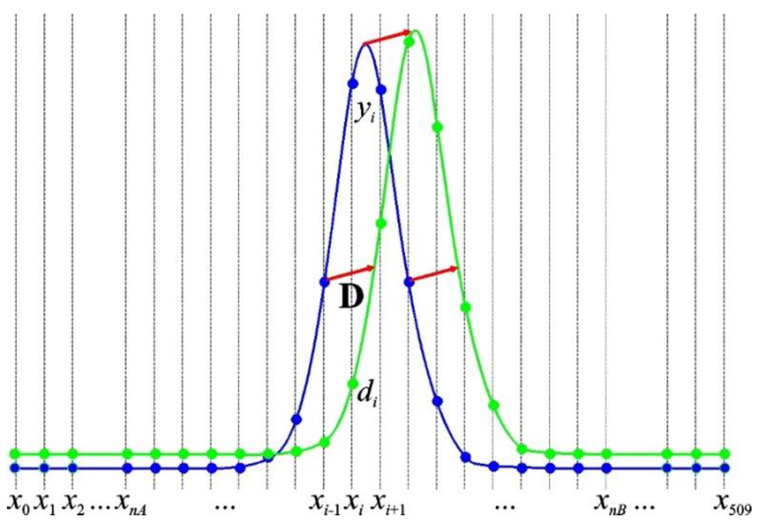
Consider a functional dependence y = f(x), which determines the magnitude of the physical impact on the sensitive element of the measuring system in the unperturbed state. At the same time, the specific form of this functional dependence is unknown. A change in the magnitude of the physical impact leads to a plane-parallel shift of the functional dependence. This shift is described as d = f(x + Δx) + Δy, where Δx and Δy are the shift parameters. Let us designate the functional dependence y(x) in the unperturbed state as the reference one, and d(x) as the shifted one. Both dependencies, y(x) and d(x), are presented with discrete data sets, {yi} and {di}, (i = 0, N), on the same uniform coordinate grid, {xi}. The grid sampling step is h = xi+1 − xi, Figure 1. The following notations are used in Figure 1: xi is the abscissa sampling set; nA is the index of the right and nB is the index of the left boundary of the controlled part of the dependence, respectively; h is the sampling step; yi are the amplitudes of the reference curve (marked in blue); di are the amplitudes of the shifted curve (marked in green); D(Δx, Δy) is the shift vector, which is the same for all points of the curve. The function f(x) can be arbitrary; however, a number of easily fulfilled requirements must be met. The function f(x) must be defined, continuous and differentiable an infinite number of times at any point x of the segment [x0, xN]. The task is to determine the shift vector D, namely the shifts, Δx, along the abscissa axis and, Δy, along the ordinate axis.
The reference and the shifted spectra are the values of the same function f(x), which is continuous and everywhere differentiable on the segment. Therefore:
Let us take advantage of the requirement that f(x) is the same function for both data sets, and it is infinitely differentiable at each point. Therefore, the values of the function f(xi + Δx) can be represented as the Taylor series near each xi:
where nD is the number of derivatives used in the approximation of the series; o(ΔxnD+1) is the remainder term of the Taylor series, the error of which has the order of (Δx)nD+1. Neglecting a small value of the remainder term of the Taylor series in Equation (2) and substituting Equation (2) into the second Equation in Equation (1), we obtain:
Equation (3) gives the system of N equations, which contains (2 + nD∙N) unknowns— namely, Δx, Δy and nD∙N derivatives f(n)(xi) (n = 1, nD and i = 1, N).
A derivative of any order can be approximated with finite-difference relations with a predetermined order over a given discrete pattern of points. For central (symmetric) finite differences on the pattern of nP = 2∙nS + 1 points {xi−nS,…, xi,…, xi+nS}, the derivative can be represented as a linear combination of the function values at the pattern points [33]:
where Ck are the coefficients of the linear combination; pi,n denotes the approximation of the n-th order derivative of the f(x) at the xi point. Central finite differences do not allow one to approximate the derivatives at the interval ends at points with indices i = 0, nS − 1 and i = N, N − nS. To approximate the derivatives at the points, which are close to end, the non-symmetric finite differences (the “forward” and “backward” finite differences, for example) can be used. However, it is possible to restrict the consideration by the controlled interval in the assumption that the controlled interval [xnA, xnB] is strictly inside [xnS, xN−nS].
The coefficients Ck of the linear combination in Equation (4) in the case of central finite differences can be found as the solution of the linear system of equations:
where A is the matrix of the linear system of equations, B is the free terms vector and C is the vector of coefficients.
Under the conditions of the above notation, the matrix A is defined as [33]:
The vector of free terms is defined as:
where nD is the derivative order, δ(x) is the delta function. All coefficients of the vector C can be calculated for an arbitrary order derivative nD on an arbitrary equidistant symmetric pattern containing nP points, provided nD ≤ nP − 1. Otherwise, the free term vector B calculated with (7) is equal to zero, and Equation (5) has a trivial solution. The approximation order of the derivative is determined with the value of (nP − nD + 1).
Thus, the reference data set {yi} (i = 0, nP−1) allows determining the derivatives pi,n up to any pre-assigned maximum order nD, calculated as finite differences on a symmetrical pattern containing nP points, at all internal grid points xi (i = nS, N − nS).
Therefore, considering the notation made and the pre-calculated derivatives, Equation (3) can be rewritten:
for all the points of the controlled area. In Equation (8), the designations for the calculated derivatives are used, and the limits of the index i, which determine all points of the controlled area, are changed versus Equation (3). As a result, Equation (8) gives (nB − nA + 1) equations for determining only two unknowns, namely Δx and Δy—the coordinates of the shift vector D(Δx, Δy). Finding a solution of the overdetermined system is carried out using the least squares method, by minimizing a convex positive definite functional:
The requirement of the minimum in Equation (9) is equivalent to the system of equations composed of two equal to zero partial derivatives of Φ(Δx, Δy) with respect to Δx and Δy:
The system of Equation (10) allows solving it regarding the unknown variables separately. The desired variable Δy can be explicitly expressed from the second Equation (10):
Substituting Δy from Equation (11) into the first Equation (10) gives an algebraic equation of one variable to determine the Δx:
Moreover, Equation (12) is a polynomial of degree 2∙nD − 1, and the solution of this equation is equivalent to finding all the roots of the polynomial T(Δx), which in a general case has exactly 2∙nD − 1 roots. An odd degree of a polynomial T(Δx) guarantees that there is at least one real root of Equation (12).
3. Algorithm
The general algorithm of the proposed approach is divided into two steps; the first of them is performed beforehand and once (Initial Step), and the second step is performed during each measurement (Regular Step).
The Initial Step consists of the following:
- -
- Determination of the odd number of pattern points nP;
- -
- Determination of the number of derivatives in the Taylor series nD;
- -
- Calculation of the coefficients C required for the derivatives’ approximation of all orders up to nD;
- -
- Single measurement with obtaining reference set {yi} at {xi} for i = 0, N;
- -
- Calculation of the derivatives pi,n (n = 1, nD) at all internal points (i = nS, N − nS).
Thereafter, the system is ready for regular operation.
The error in the approximation of derivative is determined by the value of Δx(nP−nD+1), where in Δx is the maximum shift of the spectrum from the reference position.
The Regular Step consists of:
- -
- Measurement of the shifted curve {di} (i = 0, N);
- -
- Solving Equation (12) and determining Δx—the shift of the {di} relative to the {yi};
- -
- Physical impact value calculation, using Δx.
4. Algorithm Verification
The algorithm verification was carried out on the model task of determining the shift of the central wavelength of a fiber Bragg grating. It was assumed that the fiber Bragg grating has the Gaussian shape of the reflected spectrum in the amplitude–frequency plane:
where x is the wavelength, μ0 is the central wavelength, σ is the standard deviation, yS is the minimum value, aN is the amplitude of the noise component and A is the maximum of the amplitude.
The amplitude of other-than-zero value can be chosen arbitrarily, and it does not affect the task solution. However, to make the model closer to real physical parameters, the amplitude value is taken equal to A = 104 dimensionless quantities. The amplitude of the noise component, aN, as a rule, does not exceed 0.1% of the maximum amplitude value, and the minimum value in the spectrum, ys varies in the range from 0 to 20% of the maximum amplitude value. Other simulation parameters are selected as close as possible to the operating conditions of the assembled interrogator based on the spectrum analyzer I-MON-512 [21]. Namely, the number of spectral points is N = 510; the left end of the spectral range is λMin = 1510 nm; the right end of the spectral range is λMax = 1595 nm; the sampling step of the resulting spectrum is h ≈ 0.167 nm. The central wavelength of the fiber Bragg grating is taken equal to μ0 = 1550 nm, with σ = 0.2. The maximum range of the spectrum-controlled segment is selected equal to 4 nm, which determines the indices of the left, nA = 227, and right, nB = 251, borders of the controlled segment. The maximum spectrum shift does not exceed 4 nm (μ0 ± 2 nm). The number of pattern points, nP, is varied up to 17. The maximum amount of the Taylor series, nD, is varied up to 14. It is ensured that the approximation of the derivative by finite differences is not lower than the third order of smallness.
The reflectance spectra of a fiber Bragg grating with the simulation parameters are shown in Figure 2; the blue line indicates the reference spectrum, and the green line indicates the spectrum with the shift of 0.5 nm.
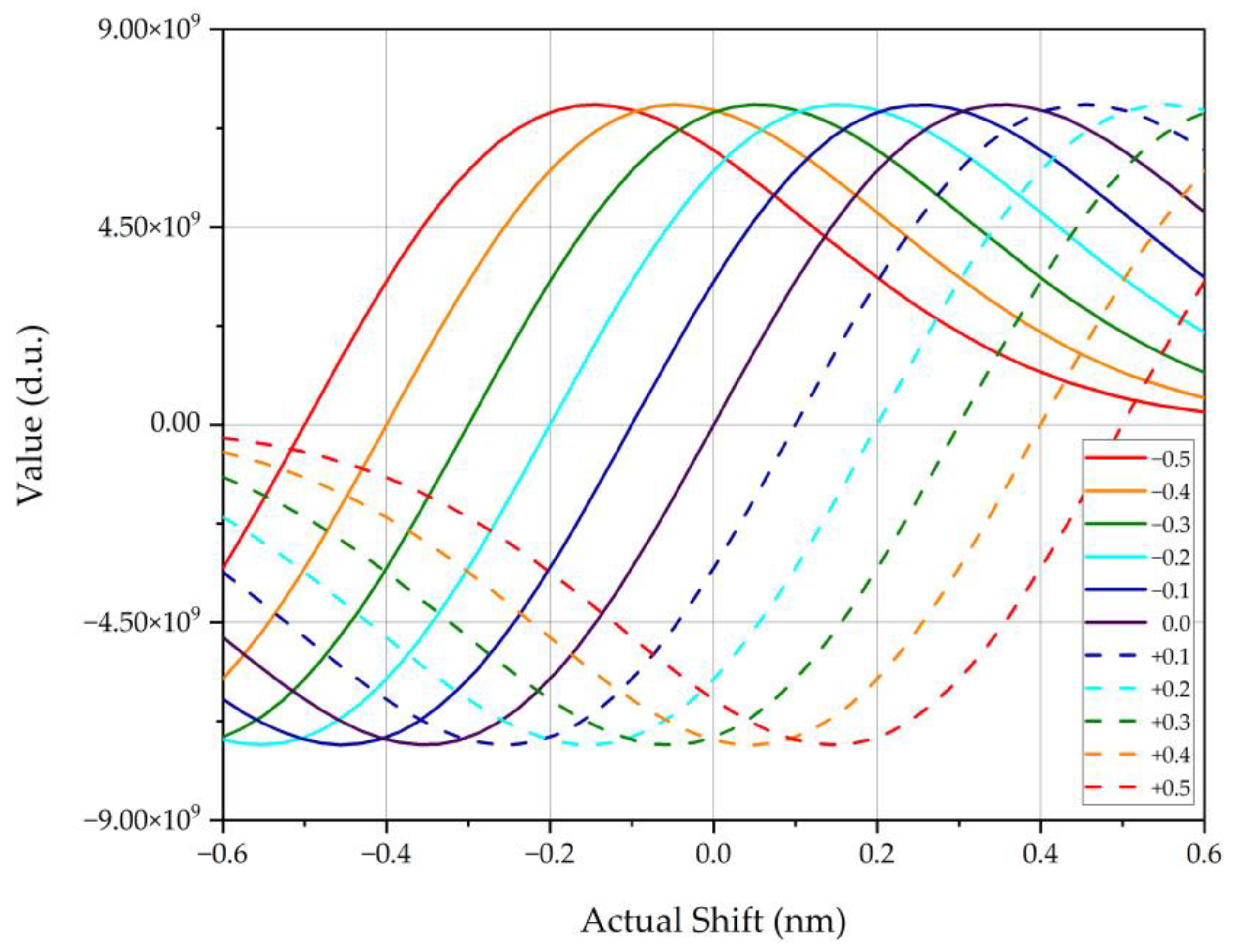
Previously, for each value of the spectrum shift with a step of 0.1 nm in the range from −0.5 to 0.5 nm, the target function T(Δx) is tabulated to determine its behavior, Figure 3. The shape of the dependence T(Δx), shown in Figure 3, guarantees the existence of a single real root of Equation (12) in the required range. Since the function T(Δx) is defined everywhere on the segment, it has different signs at the edges of the segment, hence its root in the segment can be found by the iterative bisection method. As the criterion for stopping iterations, it is necessary to use the proximity to zero of the interval for finding the root, instead of the proximity to zero of the objective function values.
Setting the requirement that the absolute error in finding the root of Equation (12) must not exceed ε = 10−14 m, let us set an arbitrary spectrum shift in the range from −0.5 to +0.5 nm. Then we generate a shifted spectrum and obtain its values at control points. Based on the data of the shifted spectrum, we calculate its shift relative to the reference spectrum. Thereafter, we build the dependence of the actual shift value on the obtained shift value based on the proposed algorithm and calculate the absolute error in the offset determination. The dependence of the absolute shift determining error on the actual shift is shown in Figure 4.
Based on the analysis of the data shown in Figure 4, one can conclude that the maximum error in the spectrum shift determination does not exceed 0.15 pm. It is one and a half orders of magnitude higher than the capabilities of most of the other methods for approximating the shift of the fiber Bragg grating central wavelength. Table 1 presents a comparison of the obtained results to the performance of existing sub-pixel techniques in similar conditions (sampling step of 156 pm and noise level of 0.1%) [20].
The best approximation results of the proposed method are obtained using the amount of the Taylor series up to 13–15 orders, with the 17-point pattern, which ensures the approximation of finite differences with an error from 2 to 4 orders of smallness. The usage of 19 or more-point patterns for approximation causes certain difficulties. In such a case, the matrix of Equation (5) is poorly defined because the determinant of the matrix is huge. Thus, the solution of the linear system of equations causes noticeable difficulties, which entails the impossibility to calculate the coefficients of the derivatives’ approximations. The usage of finite differences of the first order approximation decreases the accuracy of the method. Similar experiments with the curve shift determination in other tasks show that the proposed algorithm makes it possible to determine the spectrum shift with a resolution approximately four orders of magnitude greater than the data sampling step.
5. Algorithm Modification
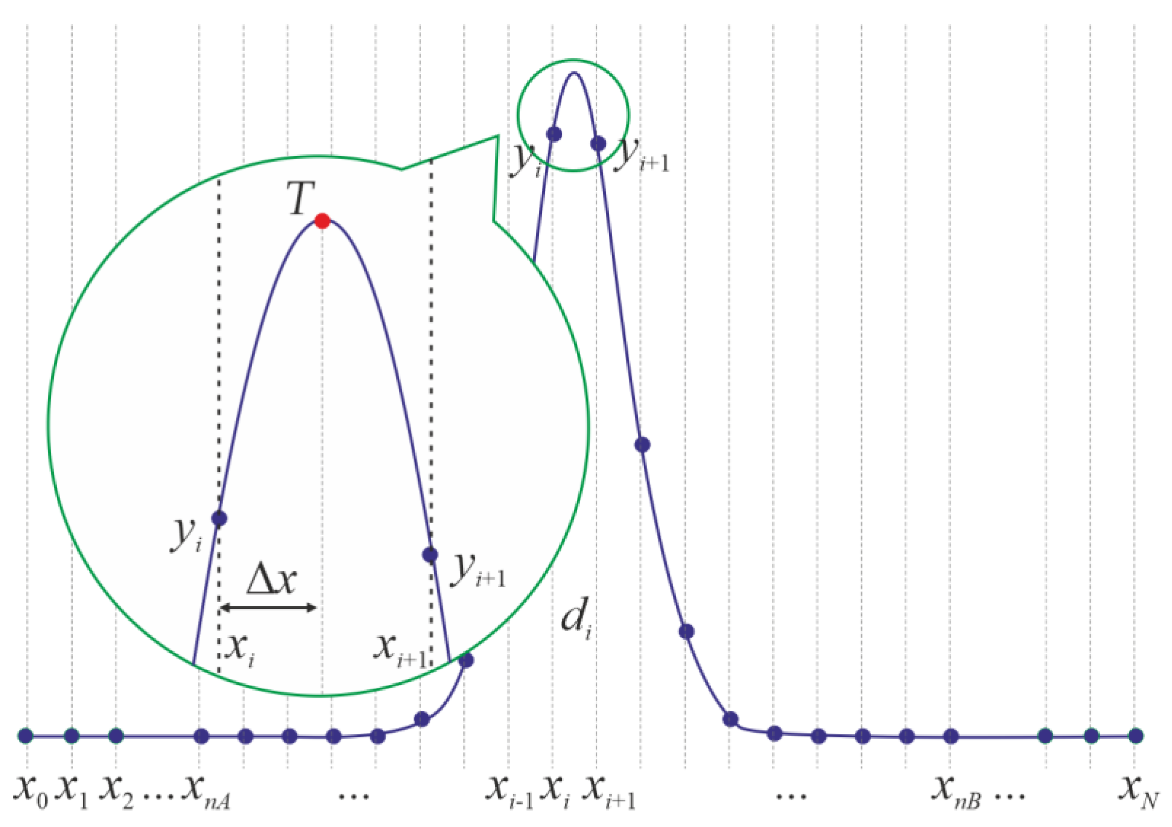
In many problems of applied physics, there is no need to solve the problem of determining the shift vector of a plane curve in the given formulation. In particular, in the problems of spectroscopy, fiber optic spectroscopy, fiber optic sensors and reflect- and refractometry, the most common task is to determine the position of the single global maximum of the curve on a selected segment with the highest possible accuracy. It allows adding one more requirement to the problem statement: let the given curve y = f(x) have only one global maximum in the segment [xnA, xnB]; moreover, the segment [xi, xi+1] of the position of the maximum has been determined in advance (Figure 5). The task is to find the position of the global maximum located inside the segment [xi, xi+1]. The value of the function at a point T arbitrarily taken inside the segment [xi, xi+1] with coordinate xi + Δx can be written according to Equation (2), where Δx ∈ [0, h] (where h is the sampling step). The problem is to find the Δx value for which the function f(xi + Δx) takes on its maximum.
This requirement means that the derivative of f(xi + Δx) with respect to Δx must be equal to zero. Differentiating the left and right parts of Equation (2) with respect to Δx and discarding terms of small orders, we obtain a nonlinear algebraic equation:
the solution of which allows us to determine the value of Δx, assuming that the value of all derivatives at the point xi is known or obtained with the finite difference method.
The presence of only one local maximum on the segment of the search for the root Δx ∈ [0, h] ensures the existence and uniqueness of the solution of Equation (14). Equation (14) is nonlinear, so its solution can be obtained only numerically.
We tested the modified algorithm under the conditions of the task. Three iterative methods (bisection, Newton–Raphson and Levenberg–Marquardt) were tested to solve it. The initial approximation for Δx was taken equal to Δx0 = h/2 for all iterative methods, which ensured a relatively fast convergence of each method. The error in the determination of the curve maximum position for all three methods turned out to be no higher (often even lower) than the same error in the determination of the shift of the curve relative to its reference position.
The modified algorithm allows one not only to reduce the computational load but also to consider the possible change in the curve shape at each measurement stage.
6. Conclusions
The proposed algorithm has numerous advantages. Firstly, it does not contain any complex calculations and can be implemented even on the simplest microcontroller. Secondly, the main computational complexity falls on the Initial Step and is performed only once. Thirdly, in the process of each measurement step, the task is only to find an existing real root of the polynomial. Fourthly, the simple bisection method can be used to solve the task, which ensures the root founding in no more than 30–35 iterations, depending on the required accuracy. Despite the apparent simplicity of the mathematical apparatus, the proposed algorithm makes it possible to increase the actual resolution of the spectrum analyzer by almost four orders of magnitude. Fifthly, the advantage of this method is its independence from the intensity fluctuations.
This method can be useful in various spectroscopic applications. For example, the chemical environment affects the Raman peak of chemical bonds; another example can be fluorescent probes, where peak shift is usually correlated with the quantity of measurements. Specifically, the fluorescence spectrum shift determination is often correlated with the broad emission spectra.
In addition, the proposed method can be applied in distributed sensing systems based on Brillouin scattering to enhance the measurement resolution. In all the mentioned applications, the current method can be used to enhance the precision of the spectrum shift determination.
The disadvantages of the proposed method are the necessity of a preliminary measurement of the spectrum and the impossibility of the central wavelength position determination of an arbitrary spectrum.
The proposed modification of the algorithm is applicable for tasks of finding the global maximum of the curve on a selected interval. The modified algorithm allows one to significantly reduce the computational load of the algorithm. Firstly, the modified algorithm does not require a reference curve, relative to which the offset is determined and, as a result, the requirement to store the reference curve in memory. Secondly, there is no need to calculate (even once) the derivatives of all orders of the reference curve at each point of the spectrum. The only requirement is to calculate derivatives of all orders at one of the points xi (or xi + 1) which is the boundary of the interval for finding the maximum. Thirdly, the modified algorithm allows one to consider the possible change in the shape of the obtained curve at each measurement stage. All these advantages make the modified algorithm very attractive for its use in spectroscopy applications.
Author Contributions
Conceptualization, A.S. and N.P.; methodology, N.P. and V.A.; software, B.V.; validation, A.N., T.A., B.V. and A.S.; formal analysis, O.M.; investigation, A.N., T.A. and B.V.; resources, O.M.; data curation, A.S.; writing—original draft preparation, A.S.; writing—review and editing, A.S.; visualization, A.S. and T.A.; supervision, N.P. and A.N.; project administration, O.M. and A.S.; funding acquisition, O.M. All authors have read and agreed to the published version of the manuscript.
Funding
This work was financially supported by the Ministry of Science and Higher Education as part of the “Priority 2030” program.
Institutional Review Board Statement
Not applicable.
Informed Consent Statement
Not applicable.
Data Availability Statement
The data presented in this study are available on request from the corresponding author.
Conflicts of Interest
The authors declare no conflict of interest.
References
- Grattan, K.T.V.; Meggitt, B.T. (Eds.) Optical Fiber Sensor Technology: Advanced Applications—Bragg Gratings and Distributed Sensors; Springer: New York, NY, USA, 2000; ISBN 978-0-7923-7946-1. [Google Scholar]
- Kronenberg, P.; Rastogi, P.K.; Giaccari, P.; Limberger, H.G. Relative Humidity Sensor with Optical Fiber Bragg Gratings. Opt. Lett. 2002, 27, 1385–1387. [Google Scholar] [CrossRef] [PubMed]
- Tai, H. Theory of Fiber Optical Bragg Grating: Revisited. In Optical Modeling and Performance Predictions, Proceedings of Optical Science and Technology, SPIE’s 48th Annual Meeting, San Diego, CA, USA, 3–8 August 2003; SPIE: Bellingham, WA, USA, 2004; Volume 5178, pp. 131–138. [Google Scholar]
- Njegovec, M.; Donlagic, D. A Fiber-Optic Gas Sensor and Method for the Measurement of Refractive Index Dispersion in NIR. Sensors 2020, 20, 3717. [Google Scholar] [CrossRef] [PubMed]
- Tseng, S.-M.; Chen, C.-L. Optical Fiber Fabry-Perot Sensors. Appl. Opt. 1988, 27, 547–551. [Google Scholar] [CrossRef]
- Chen, P.; Dai, Y.; Zhang, D.; Wen, X.; Yang, M. Cascaded-Cavity Fabry-Perot Interferometric Gas Pressure Sensor Based on Vernier Effect. Sensors 2018, 18, 3677. [Google Scholar] [CrossRef] [Green Version]
- Campanella, C.E.; Malara, P.; Campanella, C.M.; Giove, F.; Dunai, M.; Passaro, V.M.N.; Gagliardi, G. Mode-Splitting Cloning in Birefringent Fiber Bragg Grating Ring Resonators. Opt. Lett. 2016, 41, 2672–2675. [Google Scholar] [CrossRef]
- Campanella, C.E.; Leonardis, F.D.; Mastronardi, L.; Malara, P.; Gagliardi, G.; Passaro, V.M.N. Investigation of Refractive Index Sensing Based on Fano Resonance in Fiber Bragg Grating Ring Resonators. Opt. Express 2015, 23, 14301–14313. [Google Scholar] [CrossRef]
- Chen, F.; Zhang, H.; Sun, L.; Li, J.; Yu, C. Temperature Tunable Fano Resonance Based on Ring Resonator Side Coupled with a MIM Waveguide. Opt. Laser Technol. 2019, 116, 293–299. [Google Scholar] [CrossRef]
- Mandal, S.; Dasgupta, K.; Basak, T.K.; Ghosh, S.K. A Generalized Approach for Modeling and Analysis of Ring-Resonator Performance as Optical Filter. Opt. Commun. 2006, 1, 97–104. [Google Scholar] [CrossRef]
- Limonov, M.F.; Rybin, M.V.; Poddubny, A.N.; Kivshar, Y.S. Fano Resonances in Photonics. Nat. Photonics 2017, 11, 543–554. [Google Scholar] [CrossRef]
- Sakhabutdinov, A.Z.; Agliullin, T.A.; Hussein, S.M.R.H.; Kuznetsov, A.A.; Anfinogentov, V.I.; Valeev, B.I. Fano-Type Resonance Structures Based on Combination of Fiber Bragg Grating with Fabry-Perot Interferometer. Karbala Int. J. Mod. Sci. 2023, 9. [Google Scholar] [CrossRef]
- Loayssa, A.; Hernández, R.; Benito, D.; Galech, S. Characterization of Stimulated Brillouin Scattering Spectra by Use of Optical Single-Sideband Modulation. Opt. Lett. 2004, 29, 638–640. [Google Scholar] [CrossRef] [PubMed]
- Shi, X.; Zheng, S.; Chi, H.; Jin, X.; Zhang, X. Refractive Index Sensor Based on Tilted Fiber Bragg Grating and Stimulated Brillouin Scattering. Opt. Express 2012, 20, 10853–10858. [Google Scholar] [CrossRef]
- Zornoza, A.; Pérez-Herrera, R.A.; Elosúa, C.; Diaz, S.; Bariain, C.; Loayssa, A.; Lopez-Amo, M. Long-Range Hybrid Network with Point and Distributed Brillouin Sensors Using Raman Amplification. Opt. Express 2010, 18, 9531–9541. [Google Scholar] [CrossRef] [PubMed]
- Wang, C.; Yao, J. Fiber Bragg Gratings for Microwave Photonics Subsystems. Opt. Express 2013, 21, 22868–22884. [Google Scholar] [CrossRef] [PubMed]
- Qin, C.; Zhao, J.; Jiang, B.; Yang, D. Sub-Pixel Algorithms on Linear-Array Detector Grating Spectrometer. In Proceedings of the Photonics Asia conference, Beijing, China, 4–7 November 2012; Culshaw, B., Liao, Y., Wang, A., Bao, X., Fan, X., Eds.; SPIE: Bellingham, WA, USA, 2012; p. 85610N. [Google Scholar]
- Bodendorfer, T.; Muller, M.S.; Hirth, F.; Koch, A.W. Comparison of Different Peak Detection Algorithms with Regards to Spectrometic Fiber Bragg Grating Interrogation Systems. In Proceedings of the 2009 International Symposium on Optomechatronic Technologies, Istanbul, Turkey, 21–23 September 2009; IEEE: Istanbul, Turkey, 2009; pp. 122–126. [Google Scholar]
- Sakhabutdinov, A.Z.; Nureev, I.I.; Morozov, O.G. Clarification of the central wavelength FBG position in a poor signal-to-noise ratio conditions. Phys. Wave Process. Radio Syst. 2015, 18, 98–102. (In Russian) [Google Scholar]
- Tosi, D. Review and Analysis of Peak Tracking Techniques for Fiber Bragg Grating Sensors. Sensors 2017, 17, 2368. [Google Scholar] [CrossRef]
- Anfinogentov, V.; Karimov, K.; Kuznetsov, A.; Morozov, O.G.; Nureev, I.; Sakhabutdinov, A.; Lipatnikov, K.; Hussein, S.M.R.H.; Ali, M.H. Algorithm of FBG Spectrum Distortion Correction for Optical Spectra Analyzers with CCD Elements. Sensors 2021, 21, 2817. [Google Scholar] [CrossRef]
- Ruiz-Lombera, R.; Mirapeix, J.; Laarossi, I.; Rodríguez-Cobo, L.; Lopez-Higuera, J.M. Brillouin Frequency Shift Estimation in BOTDA via Subpixel Processing. In Proceedings of the Sixth European Workshop on Optical Fibre Sensors, Limerick, Ireland, 31 May–3 June 2016; SPIE: Bellingham, WA, USA, 2016; Volume 9916, pp. 366–369. [Google Scholar]
- Fleet, D.; Weiss, Y. Optical Flow Estimation. In Handbook of Mathematical Models in Computer Vision; Paragios, N., Chen, Y., Faugeras, O., Eds.; Springer: Boston, MA, USA, 2006; pp. 237–257. ISBN 978-0-387-28831-4. [Google Scholar]
- Pla, F.; Bober, M. Estimating Translation/Deformation Motion through Phase Correlation. In Proceedings of the Image Analysis and Processing, Florence, Italy, 17–19 September 1997; Del Bimbo, A., Ed.; Springer: Berlin/Heidelberg, Germany, 1997; pp. 653–660. [Google Scholar]
- Foroosh, H.; Zerubia, J.B.; Berthod, M. Extension of Phase Correlation to Subpixel Registration. IEEE Trans. Image Process. 2002, 11, 188–200. [Google Scholar] [CrossRef] [Green Version]
- Deepa, S.; Das, B. Interrogation Techniques for π-Phase-Shifted Fiber Bragg Grating Sensor: A Review. Sens. Actuators Phys. 2020, 315, 112215. [Google Scholar] [CrossRef]
- Agrawal, G.P.; Radic, S. Phase-Shifted Fiber Bragg Gratings and Their Application for Wavelength Demultiplexing. IEEE Photonics Technol. Lett. 1994, 6, 995–997. [Google Scholar] [CrossRef]
- Dai, B.; Gao, Z.; Wang, X.; Kataoka, N.; Wada, N. Performance Comparison of 0/π- and ±π/2-Phase-Shifted Superstructured Fiber Bragg Grating En/Decoder. Opt. Express 2011, 19, 12248–12260. [Google Scholar] [CrossRef] [PubMed] [Green Version]
- Morozov, O.G.; Nureev, I.I.; Sahabutdinov, A.Z.; Gubaidullin, R.R.; Morozov, G.A. Problem of Fano Resonance Characterization in Ring π-Shift Fiber Bragg Grating Biosensors. In Proceedings of the 2019 Systems of Signal Synchronization, Generating and Processing in Telecommunications (SYNCHROINFO), Yaroslavl, Russia, 1–3 July 2019; pp. 1–6. [Google Scholar]
- Xu, O.; Zhang, J.; Yao, J. High Speed and High Resolution Interrogation of a Fiber Bragg Grating Sensor Based on Microwave Photonic Filtering and Chirped Microwave Pulse Compression. Opt. Lett. 2016, 41, 4859–4862. [Google Scholar] [CrossRef] [PubMed] [Green Version]
- Ricchiuti, A.L.; Barrera, D.; Sales, S.; Thévenaz, L.; Capmany, J. Long Weak FBG Sensor Interrogation Using Microwave Photonics Filtering Technique. IEEE Photonics Technol. Lett. 2014, 26, 2039–2042. [Google Scholar] [CrossRef]
- Morozov, O.; Sakhabutdinov, A.; Anfinogentov, V.; Misbakhov, R.; Kuznetsov, A.; Agliullin, T. Multi-Addressed Fiber Bragg Structures for Microwave-Photonic Sensor Systems. Sensors 2020, 20, 2693. [Google Scholar] [CrossRef]
- Hassan, H.Z.; Mohamad, A.A.; Atteia, G.E. An Algorithm for the Finite Difference Approximation of Derivatives with Arbitrary Degree and Order of Accuracy. J. Comput. Appl. Math. 2012, 236, 2622–2631. [Google Scholar] [CrossRef] [Green Version]
Figure 1.
Scheme of physical impact on the functional dependence f(x): the reference dependence (blue line, {yi}) and the shifted dependence (green line, {di}), the shift vector D (red arrow).
Figure 1.
Scheme of physical impact on the functional dependence f(x): the reference dependence (blue line, {yi}) and the shifted dependence (green line, {di}), the shift vector D (red arrow).

Figure 2.
Spectrum of a fiber Bragg grating within the controlled wavelength range. The blue line indicates the reference spectrum; the green line indicates the shifted spectrum.
Figure 2.
Spectrum of a fiber Bragg grating within the controlled wavelength range. The blue line indicates the reference spectrum; the green line indicates the shifted spectrum.

Figure 3.
The behavior of the target function in the shift range from −0.5 to 0.5 nm for the fiber Bragg grating with a normal profile built for each shift in the range with a step of 0.1 nm.
Figure 3.
The behavior of the target function in the shift range from −0.5 to 0.5 nm for the fiber Bragg grating with a normal profile built for each shift in the range with a step of 0.1 nm.

Figure 4.
The absolute error of the shift determination.

Figure 5.
Scheme of the functional dependence f(x) (blue line) and its peak in the insert.


Table 1.
Comparison of sub-pixel processing methods in application to FBG interrogation.
| Method | Error (pm) | Resolution Increase (Times) |
|---|---|---|
| 3-dB Bandwidth | 28.7 | 5.4 |
| Centroid | 5.8 | 26.9 |
| Second-order polynomial fit | 2.2 | 70.9 |
| Gaussian fit (with resampling) | 3.7 | 42.2 |
| Karhunen–Loève transform | 0.18 | 866.7 |
| Proposed method | 0.15 | 1113.3 |
Disclaimer/Publisher’s Note: The statements, opinions and data contained in all publications are solely those of the individual author(s) and contributor(s) and not of MDPI and/or the editor(s). MDPI and/or the editor(s) disclaim responsibility for any injury to people or property resulting from any ideas, methods, instructions or products referred to in the content. |
© 2023 by the authors. Licensee MDPI, Basel, Switzerland. This article is an open access article distributed under the terms and conditions of the Creative Commons Attribution (CC BY) license (https://creativecommons.org/licenses/by/4.0/).
Share and Cite
MDPI and ACS Style
Pavlycheva, N.; Niyazgulyyewa, A.; Sakhabutdinov, A.; Anfinogentov, V.; Morozov, O.; Agliullin, T.; Valeev, B. Hi-Accuracy Method for Spectrum Shift Determination. Fibers 2023, 11, 60. https://doi.org/10.3390/fib11070060
AMA Style
Pavlycheva N, Niyazgulyyewa A, Sakhabutdinov A, Anfinogentov V, Morozov O, Agliullin T, Valeev B. Hi-Accuracy Method for Spectrum Shift Determination. Fibers. 2023; 11(7):60. https://doi.org/10.3390/fib11070060
Chicago/Turabian StylePavlycheva, Nadezhda, Ayna Niyazgulyyewa, Airat Sakhabutdinov, Vladimir Anfinogentov, Oleg Morozov, Timur Agliullin, and Bulat Valeev. 2023. "Hi-Accuracy Method for Spectrum Shift Determination" Fibers 11, no. 7: 60. https://doi.org/10.3390/fib11070060
Note that from the first issue of 2016, this journal uses article numbers instead of page numbers. See further details here.